|
Options
This Finance`Options` subpackage contains tools to compute options using the Black-Scholes model.
This loads the Options subpackage.
In[1]:=<< Finance`Options`
Here are the basic option functions.
In[2]:=?Finance`Options`*
Delta Norm
Elasticity Option
HistoricalVolatility Rho
ImpliedVolatility Theta
Lambda


An option object.
This is a put option for an asset named XYZ that expires on December 20, 1992 with an exercise (or striking) price of 40.
In[3]:=xyzft = Option[{"Put", XYZ, 40, {12, 20, 1992}}]
Out[3]=
However, we have to remember that an option is a derivative security and we need to specify the price and volatility of the underlying asset.
In[4]:=(Price[XYZ] ^= 40;
Volatility[XYZ] ^= 3/10;)
We also have to define the riskless interest rate.
In[5]:=r = 12/100
Out[5]=
We define the settlement date to be August 20, 1992.
In[6]:=settlement = {8, 20, 1992}
Out[6]=
This is a call option for an asset named ABC. The striking price is 40 and the expiration date is December 19, 1992.
In[7]:=abcft = Option[{"Call", ABC, 40, {12, 19, 1992}}]
Out[7]=
This time we specify the volatility but not the price of the underlying asset.
In[8]:=Volatility[ABC] = 3/10
Out[8]=


A basic function.
We compute the value of xyzft given the riskless interest rate r = 12%. Mathematica gives us an exact result.
In[9]:=val1 = Value[xyzft, settlement, r]
Out[9]=
Here is a numerical approximation.
In[10]:=N[%]
Out[10]=
Another way to get an approximation is to write one of the arguments with a decimal point.
In[11]:=Value[xyzft, settlement, .12]
Out[11]=
We define an option's value as a function of two variables, the price of the underlying asset x and the time to maturity t.
In[12]:=optionvalue[x_, t_] = Value[abcft,
ToCalendar[ToJulian[settlement] + Floor[t]], r] /.
Price[ABC] -> x;
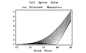
This illustrates how the graph of the option value changes as the time to maturity varies.
In[13]:=Plot[Evaluate[Table[optionvalue[x, t],
{t, 0, 120, 10}]], {x, 25, 45},
PlotLabel ->
" Call Option Value\nfor Different Maturities",
FrameLabel -> {"Stock Price", ""}];
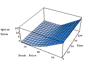
Here is the equivalent three-dimensional graph.
In[14]:=Plot3D[optionvalue[x, t], {x, 25, 55}, {t, 0, 120},
AxesLabel->{"Stock Price", "Time", "Option \nValue "}];


Sensitivity measures functions.
Here is the analytical expression for the delta of the put option xyzft.
In[15]:=Delta[xyzft, settlement, r]
Out[15]=
This is a numerical approximation.
In[16]:=N[%]
Out[16]=
We define the delta of the option abxft as a function of two variables, x and t, the price of the underlying asset and the time to maturity, respectively.
In[17]:=optiondelta[x_, t_] = Delta[abcft,
ToCalendar[ToJulian[settlement] + Floor[t]], r] /.
Price[ABC] -> x;
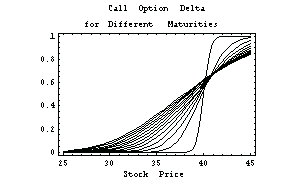
This illustrates how the graph of the option delta changes as the time to maturity varies.
In[18]:=Plot[Evaluate[Table[optiondelta[x, j],
{j, 0, 120, 10}]], {x, 25, 45},
PlotLabel ->
" Call Option Delta\nfor Different Maturities",
FrameLabel -> {"Stock Price", ""}];
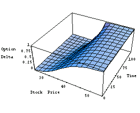
Here is the equivalent three-dimensional graph.
In[19]:=Plot3D[optiondelta[x, t], {x, 25, 55}, {t, 0, 120},
AxesLabel->{"Stock Price", "Time", "Option \nDelta"}];
Here is the analytical expression for the theta of the put option xyzft.
In[20]:=Theta[xyzft, settlement, r]
Out[20]=
This is a numerical approximation.
In[21]:=N[%]
Out[21]=
We define the theta of the option abcft as a function of two variables, x and t, the price of the underlying asset and the time to maturity, respectively.
In[22]:=optiontheta[x_, t_] = Theta[abcft,
ToCalendar[ToJulian[settlement] + Floor[t]], r] /.
Price[ABC] -> x;
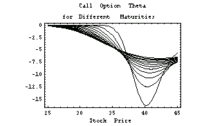
This illustrates how the graph of the option theta changes as the time to maturity varies.
In[23]:=Plot[Evaluate[Table[optiontheta[x, j],
{j, 0, 110, 10}]], {x, 25, 45},
PlotLabel ->
" Call Option Theta\nfor Different Maturities",
FrameLabel -> {"Stock Price", ""}];
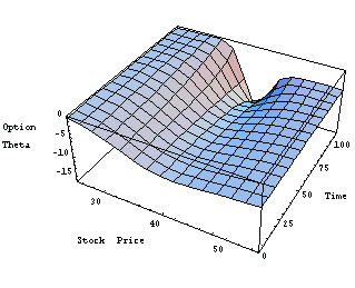
Here is the equivalent three-dimensional graph.
In[24]:=Plot3D[optiontheta[x, t], {x, 25, 55}, {t, 0, 110},
AxesLabel->{"Stock Price", "Time", "Option \nTheta"}];
Here is the analytical expression for the gamma of the put option xyzft.
In[25]:=Gamma[xyzft, settlement, r]
Out[25]=
This is a numerical approximation.
In[26]:=N[%]
Out[26]=
We define the gamma of the option abcft as a function of two variables, x and t, the price of the underlying asset and the time to maturity, respectively.
In[27]:=optiongamma[x_, t_] = Gamma[abcft,
ToCalendar[ToJulian[settlement] + Floor[t]], r] /.
Price[ABC] -> x;
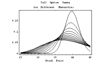
This illustrates how the graph of the option gamma changes as the time to maturity varies.
In[28]:=Plot[Evaluate[Table[optiongamma[x, j],
{j, 0, 110, 10}]], {x, 25, 45},
PlotLabel ->
" Call Option Gamma\nfor Different Maturities",
FrameLabel -> {"Stock Price", ""}];
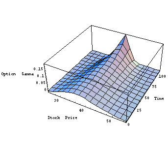
Here is the equivalent three-dimensional graph.
In[29]:=Plot3D[optiongamma[x, t], {x, 25, 55}, {t, 0, 110},
AxesLabel->{"Stock Price", "Time", "Option Gamma"}];
Here is the analytical expression for the rho of the put option xyzft.
In[30]:=Rho[xyzft, settlement, r]
Out[30]=
This is a numerical approximation.
In[31]:=N[%]
Out[31]=
We define the rho of the option abcft as a function of two variables, x and t, the price of the underlying asset and the time to maturity, respectively.
In[32]:=optionrho[x_, t_] = Rho[abcft,
ToCalendar[ToJulian[settlement] + Floor[t]], r] /.
Price[ABC] -> x;
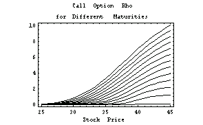
This illustrates how the graph of the option rho changes as the time to maturity varies.
In[33]:=Plot[Evaluate[Table[optionrho[x, j],
{j, 0, 120, 10}]], {x, 25, 45},
PlotLabel ->
" Call Option Rho\nfor Different Maturities",
FrameLabel -> {"Stock Price", ""}];
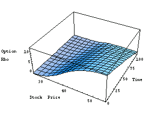
Here is the equivalent three-dimensional graph.
In[34]:=Plot3D[optionrho[x, t], {x, 25, 55}, {t, 0, 110},
AxesLabel->{"Stock Price", "Time", "Option \nRho"}];
Here is the analytical expression for the lambda of the put option xyzft. Kappa, vega, and epsilon are sometimes used instead of lambda.
In[35]:=Lambda[xyzft, settlement, r]
Out[35]=
This is a numerical approximation.
In[36]:=N[%]
Out[36]=
We define the lambda of the option abcft as a function of two variables, x and t, the price of the underlying asset and the time to maturity, respectively.
In[37]:=optionlambda[x_, t_] = Lambda[abcft,
ToCalendar[ToJulian[settlement] + Floor[t]], r] /.
Price[ABC] -> x;
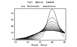
This illustrates how the graph of the option lambda changes as the time to maturity varies.
In[38]:=Plot[Evaluate[Table[optionlambda[x, t],
{t, 0, 110, 10}]], {x, 25, 45},
PlotLabel ->
" Call Option Lambda\nfor Different maturities",
FrameLabel -> {"Stock Price", ""}];
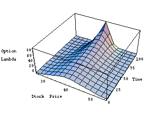
Here is the equivalent three-dimensional graph.
In[39]:=Plot3D[optionlambda[x, t], {x, 25, 55}, {t, 0, 110},
AxesLabel->{"Stock Price", "Time", "Option \nLambda"}];
Here is the analytical expression for the elasticity of the put option xyzft.
In[40]:=Elasticity[xyzft, settlement, r]
Out[40]=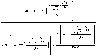
This is a numerical approximation.
In[41]:=N[%]
Out[41]=
We define the elasticity of the option abcft as a function of two variables, x and t, the price of the underlying asset and the time to maturity, respectively.
In[42]:=optionelasticity[x_, t_] = Elasticity[abcft,
ToCalendar[ToJulian[settlement] + Floor[t]], r] /.
Price[ABC] -> x;
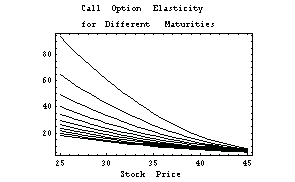
This illustrates how the graph of the option elasticity changes as the time to maturity varies.
In[43]:=Plot[Evaluate[Table[optionelasticity[x, t],
{t, 0, 100, 10}]], {x, 25, 45},
PlotLabel -> "Call Option Elasticity\n"<>
"for Different Maturities",
FrameLabel -> {"Stock Price", ""}];
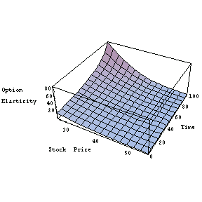
Here is the equivalent three-dimensional graph.
In[44]:=Plot3D[optionelasticity[x, t], {x, 25, 55}, {t, 0, 100},
AxesLabel->{"Stock Price", "Time",
"Option \nElasticity"}];


Implied volatility function.
This calculates the implied volatility.
In[45]:=ImpliedVolatility[xyzft, settlement, r, val1]
Out[45]=


Auxiliary functions.
To use the Black-Scholes model we need to know the underlying asset's volatility. The function HistoricalVolatility computes the maximum likelihood estimate of the asset's volatility given a list of past prices.
We read in the prices for one year of IBM stock from the file IBM-90.prc as pairs {date, price}.
In[46]:=prices[IBM] ^=
Last[Transpose[ReadList[
ToFileName[{"Finance", "Data"}, "IBM-90.prc"],
{Number, Number}]]];
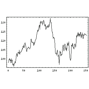
Here is the graph of IBM's prices.
In[47]:=ListPlot[prices[IBM], PlotJoined -> True];
Now we compute the maximum likelihood estimate for IBM's stock volatility. This is the daily volatility since we used daily stock prices.
In[48]:=HistoricalVolatility[prices[IBM]]
Out[48]=
To get an estimate of the yearly volatility we multiply by the square root of the number of days in a year. Usually we only take the number of trading days, which is about 250.
In[49]:=% Sqrt[250.]
Out[49]=
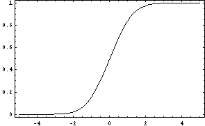
The cumulative normal distribution is often used in modern finance and especially in the context of option pricing. Here is the graph of the cumulative standard normal distribution function.
In[50]:=Plot[Norm[x], {x, -5, 5}];
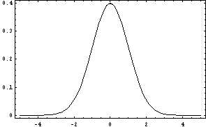
Its derivative with respect to x is indeed the standard normal distribution.
In[51]:=D[Norm[x], x]
Out[51]=
Here is the graph of the standard normal distribution.
In[52]:=Plot[Evaluate[D[Norm[x], x]], {x, -5, 5}];
|