Quick-Return

Example Mechanism for Modeler2D

by Robert Beretta

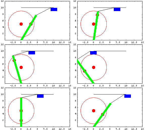
Quick Return Mechanism Animation

Discussion

Quick Return Function

This sample notebook analyzes the motion of a classic quick return mechanism using the MechanicalSystems kinematics package. This mechanism is used to demonstrate Modeler2D's basic location, velocity, and acceleration solution methods, as well as basic mechanism static and dynamic force solution methods.

Quick Return Model

The quick return mechanism consists of four bodies.
1. Ground        (black)
2. Crankshaft    (red)
3. Drive arm        (green)
4. Slider        (blue)
A real quick return mechanism would have a fifth body, the connecting link between the drive arm and the slider. However, in the kinematic model this part can be replaced by a simple distance constraint, decreasing the overall size of the model.

Each step in building the model is explained as the notebook progresses.

Kinematic Model

Preparation

The Modeler2D package is loaded into Mathematica with the Needs command.

The following symbols are used to reference each of the bodies in the quick return model.

Body Definitions

The kinematic constraints that make up the model enforce relationships between various points on the bodies of the mechanism. Each body must have a local coordinate system attached to it; the points then defined on each body are relative to that local system.

These points are defined by creating SysBody objects (hereafter referred to as body objects) with the Body function. Each body object contains all of the relevant information that is required to define a single body as follows.
1. The index number of the body. This is used to reference the body in other functions.
2. The 2D location of each point on the body, in local coordinates, given as {x, y}.
3. Initial guesses for the three degrees of freedom of the body x, y, and .
4. The mass of the body.
5. The centroidal moment of inertia of the body.
6. The location of the body's centroid, in local coordinates.

All of the items listed above, except item 1, are specified with options to the Body function and, as such, all have default values so they need not be specified. In fact, it is not necessary to use body objects at all, if none of the data they contain is relevant to the model.

Item 1, the body number, must be specified if a body object is used, and item 2, the point list, has a default value of "no points specified". Items 3-6 have default values of zero.

Ground

Four points are defined on the ground (body 1).
P1. The drive arm axis.
P2. The crankshaft axis.
P3 and P4. Two points to define the line upon which the slider slides.

Crank

Two points are defined on the crank (body 2).
P1. The crank axis.
P2. The axis of the pin that drives the drive arm.
Since the crank is a moving body, an initial guess is supplied: x -> 0, y -> 5, -> 0.

Drive arm

Two points are defined on the drive arm (body 3).
P1. The point where the drive arm pivots with the ground.
P2. The point where the drive arm is attached to the pseudo connecting link.

Slider

Two points are defined on the slider (body 4).
P1 and P2. Two points along the longitudinal axis of the slider.

Build bodies

The SetBodies command accepts the body objects as arguments and adds the information to Modeler2D's internal database.

Constraint Definitions

Now the kinematic constraints that make up the mechanism are defined. A library of simple constraints are defined by Modeler2D that return SysCon objects (hereafter referred to as constraint objects) that are recognized by the constraint building function SetConstraints.

Five constraints and one driving constraint are used to model the quick return mechanism.

Crank constraints

Constraint 1 is a revolute joint, or pivot, between the crank and the ground.

Constraint 2 is a rotational driver to turn the crank.

Note that any constraint that accepts a distance or angle for an argument can be used as a driving constraint by defining that constant to be a function of T.

Drive arm constraints

Constraint 3 is another revolute joint between the drive arm and the ground.

Constraint 4 is a translational joint between the crank and the drive arm in which the pin on the crank slides in a slot on the drive arm.

Slider constraints

Constraint 5 is a relative-distance constraint between the drive arm and the slider that replaces the pseudo connecting link.

Constraint 6 is a translational or prismatic joint between the slider and the ground.

SetConstraints accepts the constraint objects and builds the required system of equations.

Running the Model

The kinematic model is now complete. A convenient command to run before trying to run the model is CheckSystem. This tests that all of the user variables in the model are defined. If CheckSystem returns True, the model is O.K.

SolveMech[t] runs the current model at time t and, if the model converges, returns a list of rules containing the X, Y, and coordinates of each body.

The most recent list of solution rules returned by SolveMech is always given by LastSolve[].

Graphics

The next step is usually to produce some graphic output to see if the model is what we think it is. Modeler2D includes a library of graphics functions that place graphics primitives in the local coordinate system of a specified body. They parallel the built-in Mathematica graphics primitives somewhat and are defined as follows.

All of these functions return graphics objects that are functions of the model's dependent variables. The graphics objects are located by applying the current position rule, LastSolve[].

Mechanism Image

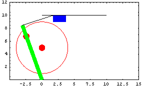
Animation

The following input generates the series of 16 graphics in the animation cell at the beginning of this notebook (don't run it unless you are prepared to wait a while).

Failure to Converge

Note that when SolveMech fails to converge on a solution and returns an error message, it implies either that the mechanism model is invalid and has no solution, or that the initial guesses are not close enough to a solution to allow Modeler2D to find it.

If SolveMech fails to converge with a mechanism that was previously working fine, it is often caused by taking too large a step in the time variable, T. Each time SolveMech searches for a new solution, it uses the last solution rule, LastSolve[] as an initial guess. If the last solution is very different from the one that is currently sought, SolveMech may be unable to find the new solution. When this happens, run SetGuess with no arguments to reset the dependent variables to their initial values and then slowly work your way towards the desired position.

For example, with this model, if SolveMech[.9] is run immediately after SolveMech[0.6], it will not converge. If SolveMech[.75] is run in between, it will.

Output

Location Output Functions

This seeks a solution to the current model at T = 0.15.

Now that an assembled configuration of the mechanism has been generated, whatever output is desired can be extracted. If information such as the location of a body's local origin is needed, it can be taken directly from the solution rule, LastSolve[].

More useful output is obtained from from a library of output functions contained in Modeler2D such as the following.

Graphing Location Output

To obtain graphic output of position as a function of time, a list of solution points is obtained using an alternate form of SolveMech.

This list of solutions can be used to generate plots of any obtainable measurement in the mechanism.

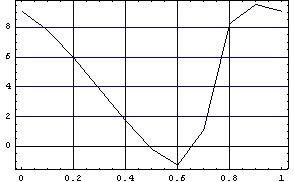
The following graphic is stored in the variable Aplot to be used later.

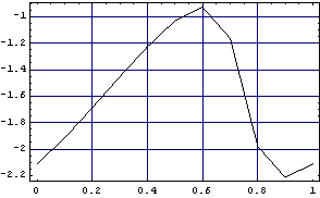
Since ListPlot connects each discreet data point with a straight line segment, the plots are not smooth. Modeler2D provides a convenient way to apply interpolation to a function.

The following graphic is stored in Bplot to be used later.

Another way to apply Mathematica's interpolation to Modeler2D is to interpolate the entire set of dependent variables with SolveMech.

SolveMech returns a list of InterpolatingFunction Rules that define the variables as direct functions of time. SolveMech accepts the option MakeRules to determine whether to return Location, Velocity, Acceleration, and/or Generalized force rules. The default MakeRules -> {Location, Parameters}, causes SolveMech to return the location solution and any parameters.

These rules can now be used for replacement with other Modeler2D output functions.

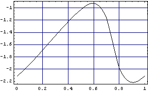
Velocity

Velocity Solution

The initial guesses should now be reset since the last time that SolveMech was called was at T = 1.0, so the current solution rule is a poor initial guess for a much smaller time.

The Solution->Velocity option causes SolveMech to build and run the velocity solution block and return the solution rule, LastSolve[], containing both the location and velocity solutions.

Velocity Output Functions

A small number of output functions for velocity are also defined.

While only a subset of the position output functions are defined for velocity output, the time derivative of any position function can be obtained with Dt.

Graphing Velocity Output

To obtain graphic output of velocity as a function of time a list of solution rules, including the velocity rules, is obtained.

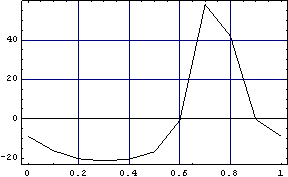
Interpolation improves the plot.

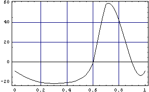
Acceleration

Acceleration Solution

The Solution->Acceleration option causes SolveMech to build and run the acceleration solution block and return the solution rule, LastSolve[], containing the location, velocity, and acceleration solutions.

Acceleration Output Functions

Output functions for accelerations are also defined.

Dt can be used twice to obtain the second time derivative of any position function.

Graphing Acceleration Output

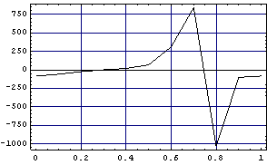
Much more accurate plots of location and velocity can be made with a small number of data points by creating an InterpolatingFunction object that includes velocity and acceleration data to define slope and curvature. TimeInterpolate and SolveMech use higher-order data automatically in the InterpolatingFunction objects they return if the higher-order terms are included in the supplied rules. Compare the following plot with the earlier ListPlot of Velocity[slider, 2]1.

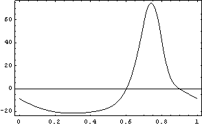
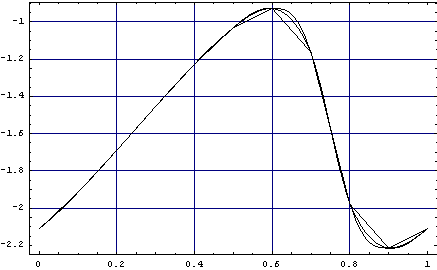
TimeInterpolate is used here to create a function that returns Angle[drivearm, 2, 1] as a function of time, using an InterpolatingFunction that includes the higher-order velocity and acceleration data. This function is more accurate than the previously created function.

Note that there is a difference between the following two interpolated plots, even though they were made with the same number of sample points. One plot uses only zeroth-order data while the other uses zeroth-, first-, and second-order data.

Loads and Reactions

Static Solutions

Loads

The forcing functions are object building functions whose return values are passed to SetLoads (just as the body and constraint objects are passed to SetBodies and SetConstraints). First, a linear spring is added to the slider.

This models a spring by making the magnitude of the force a function of distance.

Static solution

SolveMech with the Solution->Static option runs the Dynamic solution block with all velocities and accelerations set to zero, effectively rendering a static solution. Static returns the solution rule, LastSolve[], with the current values of the Lagrange multipliers appended.

Force output

The values of the Lagrange multipliers are not directly very useful, so an output function is used to find forces at the joints of the mechanism.

For example, the driving constraint, RotationLock1[2, crank, ground, 2 T], is constraint 2. The forces that are applied to the crank by constraint 2 are the forces required to enforces the driving constraint, or the forces required to drive the mechanism.

The driving constraint applies no x or y forces to body 2, because it is only a rotational constraint, and it applies 77.2 units of counterclockwise moment.

To find the x and y forces that the support for body 2 must provide, Reaction is used with constraint 1, the constraint that enforces that the axis of body 2 stay put.

Graphic force output

This creates a table of solution points through a full revolution of the crank.

This shows the torque required to rotate the crank.

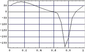
The very large negative moment spike is due to the poor leverage ratio during the quick return stroke.

Dynamic Solutions

Force output

Masses must be specified for each body for the dynamic solution to be any different from the static solution.

The Solution->Dynamic option causes SolveMech to run the Dynamic solution block with nonzero velocities and accelerations allowed and returns the solution rule, LastSolve[], with the current values of the Lagrange multipliers appended.

The same output functions are used for the Dynamic forces. Note that the reaction forces in the model are very slightly higher now than they were when considering only the static forces.

Graphic force output

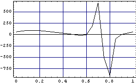
Note that the inclusion of the dynamic loads in the model only has an apparent effect at the points in time when the slider is accelerating rapidly.

Damping

If a damper is added to the slider, it may serve to reduce the high loads imposed by the spring during the return stroke.

Solution->Kinematic is used in place of Solution->Static when velocity terms are present in the forcing functions. Static simply sets the velocities to zero, while Kinematic solves for the velocities and applies the values to the forcing functions.

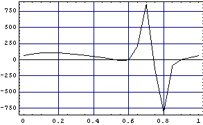
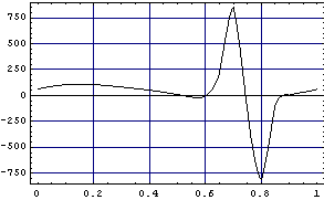
The damper seems to have evened out the reaction torque a little.

End