Space-Crank

Example Mechanism for MechanicalSystems

by Robert Beretta

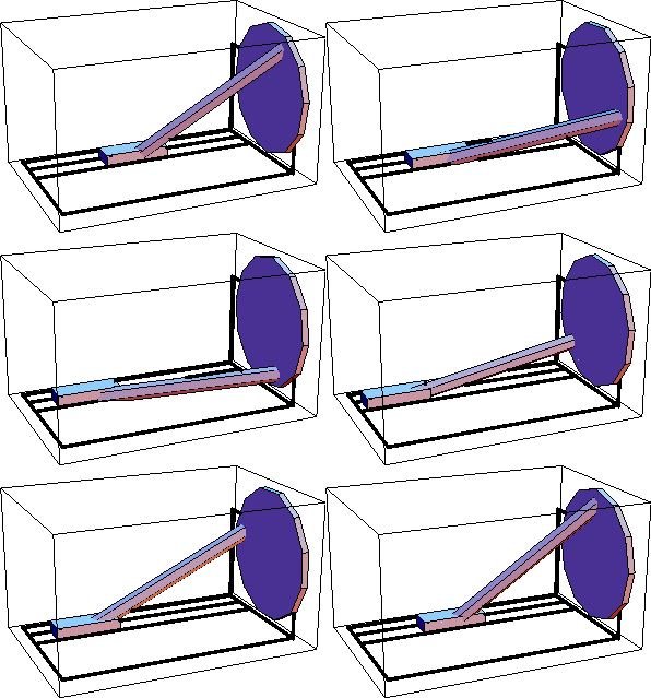
Space-Crank Animation

Discussion

Space-Crank Function

The space-crank mechanism is driven by rotating the crank, which in turn causes the slider to reciprocate via the connecting rod.

Space-Crank Model

The space-crank mechanism consists of four bodies.
1. Ground
2. Crank
3. Connecting rod
4. Slider

Kinematic Model

Preparation

The Modeler3D package is loaded into Mathematica with the Needs command.

The following names are used to reference each of the bodies in the space-crank model.

Body Definitions

Bodies are defined with the Body function, which returns a SysBody data object. The primary data that is required to define a body are the locations of the points on the body that are used to define the mechanical constraints. Other properties may also be defined with the following options.

Ground

Six points are defined on the ground (body 1).
P1. Origin of the ground body.
P2. Thr first point on the crank axis.
P3. A second point on the crank axis, slightly forward of the first.
P4. A second point (along with P1) to define the horizontal translation line of the slider.
P5. A third point (along with P1 and P2) to define the horizontal translation plane of the slider.
P6. A point that is used to define the projected angle of the crank.

Note that the InitialGuess, Mass, Inertia, and Centroid options for Body are irrelevant for body 1 because body 1 is stationary and affixed to the global coordinate origin.

Crank

Three points are defined on the crank (body 2).
P1. A point that lies on the crank axis (the local origin).
P2. A second point to define the axis of the crank (along with P1).
P3. The attachment point of the connecting rod.

The seven elements of the InitialGuess option correspond to the three location coordinates of the body and the four Euler parameters that define the rotational orientation of the body .

The six elements of the Inertia option correspond to {Ixx, Iyy, Izz, Ixy, Iyz, Izx}.

Connecting rod

Four points are defined on the connecting rod (body 3).
P1. The local origin.
P2. The upper end of the connecting rod.
P3. The lower end of the connecting rod.
P4. A second point (along with P3) to provide an orthogonal line for controlling the rotation of the connecting rod.

Slider

Five points are defined on the slider (body 4).
P1. The attachment point of the connecting rod.
P2. A second point (along with P1) to define the direction line of the translation of the connecting rod.
P3. A third point (along with P1 and P2) to define the horizontal translation plane of the slider.
P4 and P5. Points to assist in creating the graphic image.

Build bodies

SetBodies accepts the SysBody data objects and adds the information to Mech's internal database.

Constraint Definitions

Six constraints, including one driving constraint, are required to model the space-crank mechanism.

1. Revolute5. A revolute joint between the ground body and the crank. This is a five degree of freedom constraint, the one remaining degree of freedom being that the crank can rotate about an axis affixed to the ground.

2. Spherical3. A constraint between the crank and the connecting rod that constrains the end point of the connecting rod to be coincident with its attachment point on the crank.

3. OrthoRevolute4. A constraint between the connecting rod and the slider that constrains the end of the connecting rod to be coincident with its attachment point on the slider, and also constrains the the spin of the connecting rod about its axis between the slider and the crank.

4. Translate5. A constraint between the slider and the ground that allows the slider to slide in one direction only.

5. ProjectedAngle1. A constraint that gives the rotational position of the crank as a function of time.

SetConstraints accepts the SysCon data objects and adds the information to Mech's internal database.

Running the Model

The length of the connecting rod rodlength is made a parameter.

CheckSystem tests for certain mathematical errors and stray variables. A return value of True is O.K.

SolveMech[t] seeks a solution to the mechanism model at time = t.

Graphics

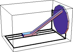
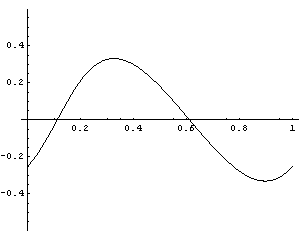
Timing

Create a table of 15 position solutions, spaced evenly from T = 0 to 1.0.

The model will run more quickly if the constraints are compiled.

The following input generates the series of 14 graphics in the animation cell at the beginning of this notebook. Do not run it unless you are prepared to wait a while, or have a fast computer.

Plots

A plot of the X position of the slider as a function of time.

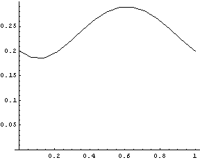
TimeInterpolate takes any expression containing Modeler3D dependent variables and a nested list of rules, such as those returned by SolveMech, and returns an InterpolatingFunction object that is a function of time.

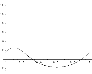
Velocity

The Solution option for SolveMech forces SolveMech to calculate velocity or acceleration terms, as well as the default location solution.

SolveMech accepts a nested list of location solution rules and updates them to velocity solutions. This is faster than recreating the location solution that has already been obtained.

Plots

A plot of the X velocity of the slider as a function of time.

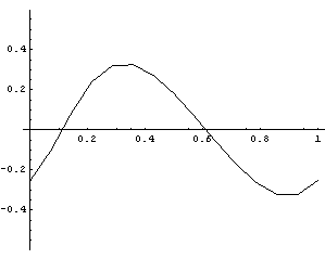
TimeInterpolate automatically includes the first-order velocity data in the interpolating function that is returned, for a more accurate interpolating function.

Acceleration

The acceleration of the slider in the X direction.

The velocity solutions are updated with acceleration data.

Plots

A plot of the X acceleration of the slider as a function of time.

TimeInterpolate automatically includes both the first- and second-order data that is contained in acctab in the returned InterpolatingFunction.

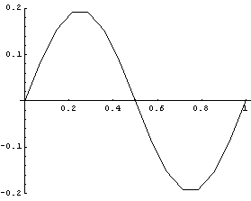
Static

To apply loads to the model, Modeler3D forcing functions are used that return SysLoad data objects, much the same as constraints and bodies are defined. The only load object that is applied at this time is Gravity, which applies a load to the centroid of each body in the current model, proportional to the body's mass.

SetLoads accepts SysLoad data objects and adds the information to Mech's internal database.

The Solution->Static option is used to force SolveMech to find the values of the Lagrange multipliers, which are used to find all of the constraint reaction forces.

The following Reaction call returns the load that constraint 1 (the Revolute5 that models the crank bearing) applies to body 1, calculated about point 1. Reaction returns forces and moments in the format {{Fx, Fy, Fz}, {Mx, My, Mz}}.

The existing table of location solutions postab is updated with the static force solution.

Plots

Here is a plot of the moment required to drive the crank, with the only applied load force being gravity, and no friction in the model. This plot should in fact be sinusoidal, because the only work that the crank is doing is lifting the weight of the connecting rod up and down in a rotary motion.

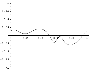
Optional Forces

Load on slider

Load on crank

Velocities

Reset

Kinematic

The Solution -> Kinematic option forces SolveMech to find the velocity solution and apply the data to the models force vector. This is only relevant if the force vector contains some velocity dependence, which the current one does not. Therefore the following input generates the same result as if Solution -> Static were used.

Dynamic

The Solution -> Dynamic option forces SolveMech to find the velocity and acceleration solutions and apply the data to the model's force vector, and calculate the inertial terms. This is only relevant if the model's force vector contains some velocity or acceleration dependence, or there are nonzero mass or inertia properties defined, which is the case in the current model.

The reaction loads at the crank bearing now have nonzero components in all directions except for moment in the X direction, which must be zero because the Revolute5 constraint does not constrain the crank against X rotation, so it can apply no moment.

The reaction forces to the driving constraint give the moment required to turn the crank.

Plots

Here is a plot of the moment required to drive the crank through one full turn.

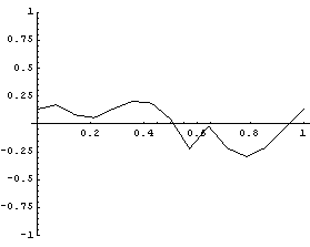
TimeInterpolate can use only first-order data, in this case, because higher-order data for the Lagrange multipliers is not present in the solution.

Saving Models

The entire state of Modeler3D can now be restored with

End