7.4 Multistage Loads

This section demonstrates how to use StageSwitch and TimeSwitch in the context of a loaded mechanism model. The use of StageSwitch and TimeSwitch in a kinematic model is covered in Chapter 5. In general, switching forces on and off is treated in the same way as switching constraints on and off.

7.4.1 Stage and Time Switches

StageSwitch

The Mech StageSwitch function is used for loads in the same manner as it is used for constraints, with one important difference. Because loads are cumulative, StageSwitch can apply more than one of the switched loads at a time, or no loads at all.

The multistage mechanism load-switching function.

Unlike most built-in Mathematica switching functions, StageSwitch does evaluate its arguments immediately. This means that test functions such as SameQ cannot be used because SameQ evaluates to True or False immediately, without waiting for some future condition to change and make it True or False in the context of the mechanism model. StageSwitch will fail if any of the test expressions fail to return True or False at runtime.
Each of the loads supplied to the StageSwitch must be a Mech load object with the head SysLoad, or a nested list of load objects.

Example

This loads the Modeler2D package.

In[1]:=

The following example shows how a StageSwitch might be used to model a force that is either a constant force in one direction or a function of T in another direction. Which force is applied is determined by the value of the user-defined symbol whichload.

Here is a valid StageSwitch load object.

In[2]:=

Out[5]=

TimeSwitch

The TimeSwitch function is also used to apply loads in much the same way it is used to apply constraints. The primary difference is that the load object TimeSwitch may have a leading time, before which no load is applied, and a trailing time, after which no load is applied.

The time-dependent, load switching function.

Each of the loads supplied to the TimeSwitch must be a Mech load object or a nested list of load objects.

Example

The following example shows how a TimeSwitch might be used to model a force applied to the slider that is to remain constraint in magnitude until the value of time reaches 2.0, at which time the force begins to increase linearly with time.

Here is a valid TimeSwitch load object.

In[6]:=

In[8]:=

Out[8]=

7.4.2 2D Example Mechanism

To demonstrate the use of Mech's StageSwitch function, a 2D model is developed that is subject to a variable applied load. The model is a simple piston-pump that has a nonlinear compression function applied to the piston.
The input to the model is to rotate the crankshaft. The pressure on the piston increases slowly but nonlinearly until near the end of its stroke, at which time the pressure decreases very rapidly back to zero. The pressure then remains at zero through the return stroke of the piston.

Here is the 2D piston-pump graphic.

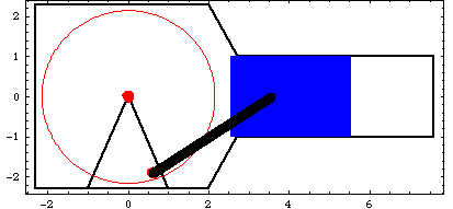
Constraints

Four constraints, one of which is a driving constraint, are required to model the piston-pump. Body objects are not defined for this model. The coordinates of the local points are simply entered directly in the point and axis objects in the constraints.

Names are defined for each of the bodies in the model.

In[9]:=

Here are the constraint objects for the model.

In[12]:=

Here is a reasonable initial guess for the piston.

In[17]:=

Loads

Only one load is applied to the piston-pump model, but this one load will be a two-stage StageSwitch load. Since the piston is initially at the top of its stroke and proceeds toward the bottom, there is no load on the piston for the first half turn of crank rotation. The two segments of the StageSwitch load are defined as follows.

Here are the two forces on the piston.

In[18]:=

The StageSwitch load must switch between f1 and f2 at the proper time. This is done by testing the value of the X coordinate of the piston X3 and the angular coordinate of the crank 2.

Here is the StageSwitch load object for the pump.

In[20]:=

Out[20]=

The loads are incorporated into the model.

In[21]:=

Running the Model

The loaded model can now be run with the Solution -> Static option for SolveMech. Note that all of the loads are zero at T = 0.1 because the force is turned off.

Now run the model at T = 0.1.

In[22]:=

Out[22]=

Here is the piston-pump model at T = 0.1.

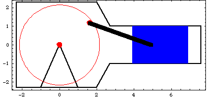
By creating a large table of solution points, plots can be made of various forces, moments, and reactions in the model using ListPlot.

Here is a list of 81 solutions.

In[23]:=

The Loads function returns the total load on the piston.

In[24]:=

Out[24]=

The force on the piston can be plotted as a function of piston travel.

In[25]:=

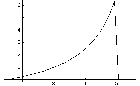
Out[25]=

The reaction forces at the constraints can be found with the Reaction function. Constraint 4 is the RotationLock1 driving constraint, so its reaction is the moment applied to the crank. Constraint 1 is the Revolute2 constraint that positions the crank axis, so its reactions are the X and Y forces supporting the crank axis.

Here is the moment required to rotate the crank.

In[26]:=

Out[26]=

Here is the reaction at the crank as a function of time.

In[27]:=

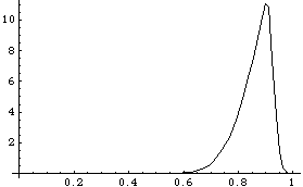
Out[27]=

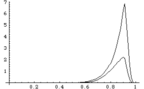
Because ListPlot is not able to plot two lists simultaneously, Mathematica graphics primitives are used directly to plot the X and Y reactions.

Here are the X and Y reaction forces at the crank axis as a function of time.

In[28]:=

Out[28]=

Undocumented Graphics Generation