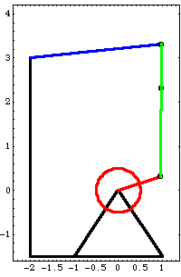
9.1 Coupled ModelsThe simplest invocation of the SetCouple and SolveCouple functions is to allow a model parameter or parameters to be varied in an attempt to satisfy some geometric condition at one point in time. In this section a planar model of a four-bar mechanism is developed, and the lengths of the links in the four-bar mechanism are adjusted to achieve various desired geometric design goals. 9.1.1 2D Example MechanismThis subsection develops a planar model of a classic four-bar mechanism. The driving input to the model is to specify the rotation of bar 2, the drive bar. Because the drive bar is the shortest link in the model, the driven bar and center bar simply oscillate as the drive bar progresses through each full turn. Driven in this manner the model has no singular configurations. This loads the Modeler2D package. Here is a graphic of the four-bar model.

BodiesFour body objects are defined for the four-bar mechanism model. Each body in the model is simply a two-ended bar, so only two local points are defined on each body. Each body is attached to one neighboring body at its local origin and another neighboring body at an offset point on the local x or y axis. Body 4, the center bar, has a third point defined that is used only as a point of reference to measure the motion of the model.
The body objects are defined such that the length of each bar is a symbolic parameter that can be changed at a later time. Names are defined for each of the body numbers in the model. Here are the four body objects for the four-bar model. The body objects are incorporated into the current model with SetBodies. ConstraintsFive constraints, one of which is a driving constraint with explicit dependence on time, are used to model the four-bar mechanism. A RotationLock1 constraint controls the rotation of the drive bar as a function of T. Four Revolute2 constraints model the revolute joints at each end of the four bars. Here are the five constraint objects for the four-bar model. The constraint objects are incorporated into the current model with SetConstraints. RuntimeBefore the model can be run, the symbols bar2, bar3, and bar4 that determine the length of the each bar must be defined. The SetParameters function is used to make the symbols formal parameters so that they are recognized by SetCouple. The symbolic lengths of each bar are defined.
Out[20]= |  |
Now the model is run at T = 0.05.
Out[21]= |  |
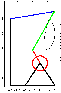
Here is a plot of the four-bar mechanism with the locus of a point on the center bar.

9.1.2 Solving for One ParameterThe coupled system building and solving functions. Mech's SetCouple and SolveCouple functions are now used to adjust the length of the drive bar bar2. In the four-bar's current configuration, the X coordinate of point 3 on the center bar is 0.898 at T = 0.1. The following example uses a coupled system to find the length of the drive bar that causes the X coordinate of point 3 to be equal to 0.8 at T = 0.1. Here is the current X coordinate of point 3 on the center bar.
Out[23]= |  |
SetCouple basically adds a degree of freedom to the mechanism model by allowing a parameter to become a dependent variable, and also adds an equation to constrain the new degree of freedom. The following command essentially says "adjust the value of bar2 such that the X coordinate of point 3 on the center bar is equal to 0.8 at the current default time T = 0.1."
The current default initial guesses obtained from LastSolve[] are used as the initial guesses for the CoupleSystem, unless otherwise specified. The current value of the parameter bar2 is used for its initial guess. This builds the CoupleSystem object.
Out[24]= |  |
SetCouple returns a CoupleSystem object that is solved with SolveCouple. The CoupleSystem object contains a new set of constraint equations that include all of the constraints in the current model, plus one. The list of rules returned by SolveCouple is of the same form as the rules returned by SolveMech. This solves the CoupleSystem object and finds a new value of bar2.
Out[25]= |  |
The new value of the parameters bar2 is added to the current parameters list.
Out[26]= |  |
This shows that the desired condition is satisfied.
Out[27]= |  |
Options for SolveCouple. Without building a new CoupleSystem object, cpsys can be re-solved at a new value of time by using the InitialCondition option. Note that the InitialCondition option expects a setting of the form Time -> t, not T -> t. The CoupleSystem is solved again with a new value of time.
Out[28]= |  |
The contents of the current parameters list are updated.
Out[29]= |  |
9.1.3 Solving for Multiple ParametersBuilding coupled systems with multiple parameters. Multiple parameter values are solved for by supplying an equal number of geometric conditions to be satisfied. A coupled system is used here to find the values of bar2 and bar3 that simultaneously cause the X coordinate of point 3 on the center bar to be 0.8 and the distance from the global origin to point 2 on the center bar to be 3.5, both at T = 0.1. This finds the X coordinate of point 3 and the distance from the origin to point 2 at T = 0.1.
Out[30]= |  |
This builds the CoupleSystem object.
Out[31]= |  |
This solves the CoupleSystem object and finds new values for bar2 and bar3.
Out[32]= |  |
This shows that the desired conditions have been satisfied.
Out[33]= |  |
In all the preceding examples, the value of time T at which the coupled model has been solved has been taken from the default initial guess list. The Time option is used to explicitly set the value of time in the CoupleSystem object, or to specify that time is a dependent variable. An option for SetCouple. Instead of fixing time at 0.1, time can be a dependent variable to be solved for. The following example seeks the values of bar2 and T that satisfy the same pair of conditions that were used in the previous example. The parameter bar3 is reset to its original value before building the new CoupleSystem.
Out[35]= |  |
Here is the solution for T and bar2.
Out[36]= |  |
The desired conditions are satisfied.
Out[37]= |  |
Undocumented Graphics Generation
|