10.1 Equilibrium ConfigurationThis section describes the use of the SetFree and SolveFree functions to find the equilibrium configuration of an underconstrained mechanism subject to static forces. A planar model of a pendulum sliding on a massless rope is used to demonstrate the use of SetFree and SolveFree. 10.1.1 Example MechanismThe pendulum-on-a-rope model in the following example consists of two planar bodies, a slider that moves without friction along an infinitely flexible, inextensible, massless rope, and a pendulum that hangs below the slider and is attached to the ground by a spring. Before an equilibrium analysis can be done, the model must have a full set of kinematic constraints so that it can be assembled and each body can be moved to a reasonable position to use as an initial guess for the equilibrium analysis. Some of these kinematic constraints are then dropped to make the model underconstrained. This loads the Modeler2D package and turns off the general spelling warnings. BodiesThree body objects are defined for the pendulum model. Note that the zeroth point, which is defined to be {0,0} by default, is used in each body. The ground (body 1) requires three point definitions.
P0 is the origin of the ground body and the attachment point of the left end of the rope.
P1 is the attachment point of the right end of the rope.
P2 is the attachment point of a spring that is used to pull the pendulum to one side.The slider (body 2) requires three point definitions.
P0 is the origin of the slider and the point where the pendulum is attached.
P1 is the point where the rope exits the left side of the slider.
P2 is the point where the rope exits the right side of the slider.The pendulum (body 3) requires two point definitions.
P0 is the origin of the pendulum and its center of mass.
P1 is the point where the pendulum is attached to the slider.Names are defined for each of the body numbers. Here are the three body objects, including inertia properties. ConstraintsSeven constraints are used to model the pendulum-on-a-rope model. A RelativeDistance1 constraint is used to model the left side of the rope. Since only the total length of the rope is known, the distance from the left end of the slider to the attachment point of the rope on the ground is simply constrained to be the unknown s. The symbol s is then added to the model as a dependent variable with the Constraint function.Another RelativeDistance1 constraint models the right side of the rope. The length of the right side of the rope is simply the total length of the rope minus the length of the slider and the length of the left side, 5 - 1 - s.A Constraint function is used only to introduce the variable s, and its initial guess, into the model as a dependent variable. The Constraint has no constraint equation, so it constrains zero degrees of freedom, but it does add one degree of freedom to the model by introducing s.A Revolute2 constraint attaches the pendulum to the slider.A RelativeX1 constraint initially controls the X coordinate of the slider. This constraint is dropped for the equilibrium analysis.A RotationLock1 constraint initially controls the rotation of the slider. This constraint is dropped for the equilibrium analysis.A RotationLock1 constraint initially controls the rotation of the pendulum. This constraint is dropped for the equilibrium analysis.Here are the seven constraint objects for the pendulum-on-a-rope model. RuntimeBecause there is no occurrence of time T in the model, the model can be run with the SolveMech command with no time argument. Since there are no other symbolic parameters, the model can only achieve one configuration, the one specified by the constraints. Now the model is run with SolveMech.
Out[9]= |  |
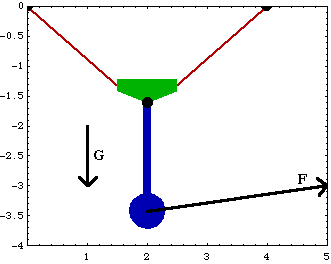
Here is the pendulum-on-a-rope model in its initial configuration.

ForcesA model must have some nonzero loads applied to it in order to have a unique equilibrium position. The pendulum-on-a-rope model has three forces applied to it: a spring force applied to the pendulum, and gravity applied to the pendulum and the slider. Here are the loads applied to the pendulum and slider. Here is the reaction to constraint 7 that prevents the pendulum from rotating. The constraint applies a clockwise moment to the pendulum to constrain it against the force of the spring.
Out[11]= |  |
10.1.2 Finding EquilibriumTo find the equilibrium configuration of a mechanism, a FreeSystem object is built that contains a new set of equations of motion with one or more constraints removed from the model. Finding equilibrium configuration. The pendulum-on-a-rope model has three constraints that are present only to complete the kinematic model, constraints 5, 6, and 7. Each of these constraints is dropped, one at a time, and the equilibrium position is found with each new degree of freedom. The first constraint to be dropped is constraint 7, which locks the rotation of the pendulum relative to the slider. This allows the pendulum to rotate, but the slider stays locked at the center of the rope. This drops constraint 7.
Out[12]= |  |
This solves the FreeSystem object.
Out[13]= |  |
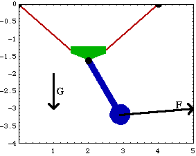
Here is the pendulum model with constraint 7 dropped.

Next, constraint 5 is dropped, allowing the slider to move along the rope. Finally, constraint 6 is dropped, allowing the slider to rotate. The InitialGuess option is used to pass SetFree the solution to the last FreeSystem, which is named sol. This solution is a better initial guess than the defaults pulled from LastSolve[]. An option for SetFree. Here is another FreeSystem object with constraints 5 and 7 dropped. This solves the FreeSystem object. Note that X2 has increased because the slider has moved to the right.
Out[15]= |  |
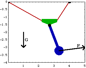
Here is the equilibrium position with constraints 5 and 7 dropped.

Here a FreeSystem object with constraints 5, 6, and 7 dropped is built and solved.
Out[17]= |  |
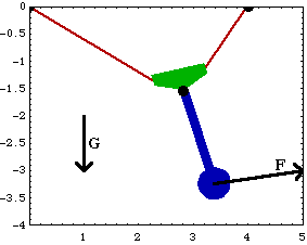
Here is the complete equilibrium position of the pendulum-on-a-rope model.

This returns MechanicalSystems to its initial state. Undocumented Graphics Generation
|