For any p × p transfer-function matrix G(s), evaluated at some frequency s = j , a corresponding comparison matrix M can be defined as , a corresponding comparison matrix M can be defined as where the elements mij are the moduli of the corresponding elements of the matrix G. By definition, the comparison matrix M is element-wise nonnegative. A normalized form of M can be constructed as where  = diag{mii}. If = diag{mii}. If  is square, positive, and irreducible, that is, there is no permutation matrix P such that is square, positive, and irreducible, that is, there is no permutation matrix P such that where X and Z are square matrices, then there exists an eigenvalue of  called the Perron-Frobenius eigenvalue, called the Perron-Frobenius eigenvalue,  pf, that is always real and positive. Furthermore, if the eigenvalues are ordered so that | pf, that is always real and positive. Furthermore, if the eigenvalues are ordered so that | 1| 1|  | | 2| 2|  ... ...  | | p|, then p|, then  pf > pf >  i for i ≠ 1. i for i ≠ 1. If  pf < 2, then pf < 2, then is both row and column diagonal dominant at s = j , and in a nearby neighborhood, and the required scaling matrix S-1 is formed from the elements of the corresponding Perron-Frobenius right eigenvector wpf of , and in a nearby neighborhood, and the required scaling matrix S-1 is formed from the elements of the corresponding Perron-Frobenius right eigenvector wpf of  , as , as When working with the inverse system, Eq. (5.NumberedEquationNormalized M) is replaced by and the matrix S is formed from the elements of the corresponding Perron-Frobenius left eigenvector wpf of  . . If a constant input scaling compensator, as defined by Eq. (5.NumberedEquationPerron-Frobenius scaled G), is implemented, then the same dominance ratio, introduced in Section 5.2.3, is obtained in all diagonal elements of the resulting Nyquist array at the design frequency s = j . The best row (or column) dominance ratio that can be achieved with a constant diagonal scaling compensator is given by . The best row (or column) dominance ratio that can be achieved with a constant diagonal scaling compensator is given by  pf(j pf(j )-1. )-1. You should note that although the compensator designed using the Perron-Frobenius approach is implemented as an input-scaling compensator, manipulating the columns of the Nyquist array, it attempts to achieve the best row diagonal dominance. A plot of the Perron-Frobenius eigenvalue with frequency is therefore a useful scalar indicator of the level of interaction, or diagonal dominance, in a system that can be achieved by implementing a diagonal input-scaling compensator. The function PerronFrobeniusEigenvaluePlot generates this plot. | PerronFrobeniusEigenvaluePlot[system] |
| | plot the Perron-Frobenius eigenvalue for system |
| PerronFrobeniusEigenvaluePlot[system, {w, wmin, wmax}] |
|
| | plot the Perron-Frobenius eigenvalue for system for frequency w running from wmin to wmax |
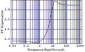
Creating the Perron-Frobenius eigenvalue plot. Make sure the application is loaded. This is the two-input, two-output transfer-function object, considered earlier. | Out[3]= |  |
The direct-system Nyquist array of this system, determined in Section 5.2.1, was found not to be diagonal dominant, and a first step in the design of a compensator for this system might be to determine whether, or not, it can be made diagonal dominant using a simple diagonal constant input-scaling compensator. This creates the Perron-Frobenius eigenvalue plot for the transfer-function object. 
Since the Perron-Frobenius eigenvalue is less than 2 over the bandwidth of interest, the system can be made diagonal dominant at any frequency in this bandwidth, and in the nearby neighborhood, by a simple constant diagonal scaling matrix.
The function PerronFrobeniusCompensator can be used to determine such a compensator. | PerronFrobeniusCompensator[system] |
| | calculate a Perron-Frobenius constant diagonal scaling compensator for the object system at zero frequency |
| PerronFrobeniusCompensator[system, w] |
|
| | calculate a Perron-Frobenius constant diagonal scaling compensator for the object system at the frequency w |
The Perron-Frobenius constant compensator functions. This determines a Perron-Frobenius constant scaling compensator at zero frequency. | Out[6]= |  |
This applies the compensator to the system. | Out[8]= |  |
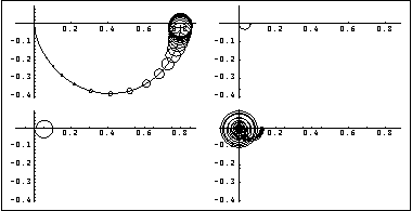
Here is the resulting Nyquist array. 
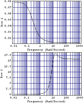
Comparing this with the Nyquist array plot in Section 5.2.1, you can see that this compensator has significantly improved the low-frequency row diagonal dominance of element {1, 1} of the Nyquist array, but has made the high-frequency row diagonal dominance of element {2, 2} much worse. With this input scaling compensator, the row dominance ratio that will be achieved in both diagonal elements of the Nyquist array at zero frequency is  pf(0)-1. Since pf(0)-1. Since  pf(0) is 1.079, the best row dominance ratio at zero frequency is 0.079. pf(0) is 1.079, the best row dominance ratio at zero frequency is 0.079. This can be confirmed by applying the function RowDominanceRatioPlot, introduced in Section 5.2.3, to the scaled system. 
While the dominance ratio in each row is 0.08 at  = 0 rad/s, as predicted, the dominance ratio of row 2 at the intermediate and high frequencies is unacceptable, and a scaling compensator at another frequency might yield better results. = 0 rad/s, as predicted, the dominance ratio of row 2 at the intermediate and high frequencies is unacceptable, and a scaling compensator at another frequency might yield better results. |