While pole assignment using state feedback provides a powerful means of changing the behavior of a given system, it assumes that all the system state variables are available for feedback. As this is not usually the case, some means of obtaining good estimates of the system state variables from the available measurements is normally required in order to be able to apply these techniques. Full state reconstruction is introduced in Section 9.2 of Control System Professional. Here, the use of the reduced-order estimator (also known as the Luenberger observer) is considered, as this can be used to reconstruct those state variables that cannot be recovered directly from the system outputs. The reduced-order state estimator described in Patel and Munro (1982) is based on the Luenberger observable canonical form of the system, which is described in Section 6.4. A similar approach is described in Chapter 6 of Advanced Numerical Methods. Given an n"th"-order linear system in state-space form with q outputs and p inputs, then a reduced-order dynamical system of order n-q, called an estimator, can be constructed with state vector z such that z approximates a linear combination of n-q of the system states given by where L has dimensions (n-q) × n. An observer of order n-q is then defined for the system of Eq. (6.8) by where F, G, and H are matrices of constants with dimensions (n-q) × (n-q), (n-q) × p, and (n-q) × q, respectively. The desired estimate  of the system state vector x is then recovered from z and the system outputs y as of the system state vector x is then recovered from z and the system outputs y as where The observer, as described by Eqs. (6.10-6.12), is the same as that described in Section 6.2 of Advanced Numerical Methods as where the matrix F corresponds to the matrix Ao, the matrices G and H are contained in the block-matrix Bo, the matrix K2 corresponds to the matrix Co, and the block-matrix [K1 0] corresponds to the matrix Do. The design of the observer requires the solution of the observer equation such that the matrix L has maximum rank, in order to guarantee the recovery of the unmeasurable state variables. Thus, not only must L have maximum rank, but the matrix  must also have maximum rank, since K1 and K2 are determined from must also have maximum rank, since K1 and K2 are determined from The reduced-order estimator algorithm developed by Munro (Patel and Munro (1982)) is based on the Luenberger observable canonical form of the system, discussed in Section 6.4.2. To determine a reduced-order estimator for a given system, you simply have to specify the dynamics of the observer, that is, the n-q eigenvalues of the matrix F. Here, these do not need to be distinct, as is the case with other reduced-order observer algorithms, but must be chosen to be faster than the fastest eigenvalue of the system matrix A. An advantage of this algorithm is that the designer can specify exactly the speed with which the observer tracks the system states. It can also deal with systems containing symbols. The function ReducedOrderEstimator implements this approach and returns the state-space system where the observer, with inputs {y,u}T and outputs  , is connected to the system as shown in Figure 6.1. , is connected to the system as shown in Figure 6.1. 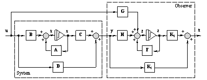
Figure 6.1. System with observer. | ReducedOrderEstimator[system, poles] |
| | determine a reduced-order observer, with the specified poles |
Reduced-order estimator. Make sure the application is loaded. Consider a fourth-order state-space system with two inputs and two outputs. | Out[3]= | 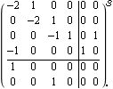 |
These are the open-loop system eigenvalues. | Out[5]= |  |
Since there are q = 2 outputs, and the rows of the matrix C are linearly independent, a reduced-order estimator of order no=n-q=2 can be constructed. This finds the reduced-order estimator for the system, with eigenvalues {-3, -4}. | Out[7]= | 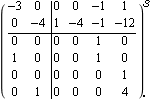 |
The system has two inputs. | Out[9]= |  |
This connects a dummy identity block I in parallel with the system ss, to allow the system inputs to be connected to the observer. | Out[11]= | 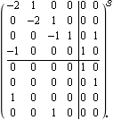 |
This connects the observer in series with the system ss1. The outputs 1 and 3 of the resulting system provide a direct measurement of states 1 and 3, respectively. | Out[13]= | 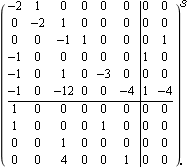 |
The eigenvalues of the combined system are the union of the eigenvalues of the closed-loop system and the state estimator. This property is known as the separation principle. This verifies the separation principle. | Out[15]= |  |
This sets the system inputs to apply a unit-step function only to input 2. This sets the initial conditions for the basic system ss. This generates the responses of the system states x2 and x4, when the system is released from the initial state x0, with input u. This sets the initial conditions for the basic system with observer, ss2. This generates the estimates of the system states x2 and x4, as produced by the observer. This compares the actual responses of the system states x2 and x4 (shown as solid lines), with the estimated values (shown as dashed lines). 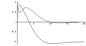
The responses of the state variables x1 and x3 are not shown, as these states are reconstructed directly from the system outputs. However, as you can see, the observer (starting from zero initial conditions) rapidly locks on to the two states being estimated, and then faithfully tracks them. Since the Luenberger canonical form functions can deal with symbolic matrices, you can also obtain the generic solution to a reduced-order estimator design. This is the state-space model of the inverted pendulum from Section 9.2 of Control System Professional. | Out[23]= | 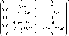 |
As it is a single-input system, there is only one observability index. | Out[25]= |  |
This is the Luenberger observable form of the system. | Out[27]= | 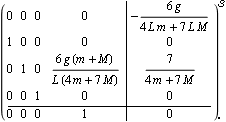 |
Here is the generic form of the reduced-order observer with all poles at p. | Out[29]= | 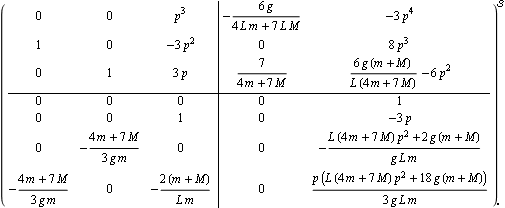 |
This is the resulting observer for a particular set of numerical values. | Out[31]= | 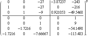 |
|