LeftMatrixFraction creates a left matrix-fraction model of a system from the denominator and numerator matrices, or another control object. | | create a left matrix fraction with denominator matrix d and numerator matrix n, in the formal variable # |
| LeftMatrixFraction[var, d, n] |
| | create a left matrix fraction with denominator matrix d and numerator matrix n, in the variable var |
Left matrix-fraction data structure. Make sure the application is loaded. Here are two polynomial matrices describing a left matrix-fraction model. Note that a matrix fraction does not necessarily have a matrix D that is diagonal. | Out[3]= |  |
| Out[5]= |  |
LeftMatrixFraction keeps its component matrices unchanged. | Out[7]= |  |
This is the TraditionalForm of the same object. | Out[9]= |  |
This output format shows one object that consists of two matrices. The first contains the inverse of the denominator matrix D(s), and the second contains the numerator matrix N(s). The | indicates that these two matrices constitute a LeftMatrixFraction object.
Similarly to other polynomial control objects, you can apply the LeftMatrixFraction object to a variable to extract the underlying matrices in that variable. indicates that these two matrices constitute a LeftMatrixFraction object.
Similarly to other polynomial control objects, you can apply the LeftMatrixFraction object to a variable to extract the underlying matrices in that variable. This produces a list of the matrices D and N in the variable s. | Out[11]= |  |
A left matrix-fraction model can also be created from an existing system model in transfer-function, zero-pole-gain, state-space, system matrix, or right matrix-fraction (see Section 3.4.2) form. | LeftMatrixFraction[system] |
| | create a left matrix-fraction object of a system |
| LeftMatrixFraction[var, system] |
| | create a left matrix-fraction object in the specified variable var |
Left matrix-fraction object data structure for converting from other system forms. Here is a StateSpace object. | Out[13]= |  |
This constructs a left matrix-fraction object. Since no formal variable is supplied, the result is obtained in the pure function form, that is, in the variable #. | Out[15]= |  |
You can also construct a LeftMatrixFraction object in the variable of your choice. | Out[17]= |  |
In TraditionalForm, both systems use the same variable  . . | Out[19]= |  |
A left matrix-fraction object can be transformed to any other model form by applying the appropriate wrapper. Here is a TransferFunction object. | Out[21]= |  |
This is the corresponding LeftMatrixFraction. | Out[23]= |  |
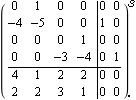
This is a corresponding SystemMatrix model. | Out[25]= |  |
The result highlights the correspondence between the system matrix object in left-fraction form and the left matrix-fraction object. Since the matrix T of the system matrix object is diagonal, it is easy to see that the model concerned is fourth-order, which corresponds exactly with the degree of the determinant of the left matrix-fraction model. This would also be the order of a minimal state-space realization. This is a state-space realization of the system. | Out[27]= |  |
The fourth-order realization is both controllable and observable and, therefore, minimal. | Out[29]= |  |
|