|
Chapter 6
Analysis of Stress
6.1 Introduction
With the Structural Mechanics functions, you can obtain a large spectrum of information about the stress state at a point in a deformable body. Mathematically, the state of stress at a point in an elastic body is determined by six independent stress components and is specified by a second-order symmetric Cartesian tensor, also known as the stress tensor. The values of these stress components change with the orientation of the coordinate system in which each stress component is defined. You can rotate the coordinate system so you can study some of the practical issues of the stress state at a point. For example, you can reduce certain stress components to zero in a particular orientation of the coordinate system. Such information is useful in calculating the stress concentrations in a stress analysis.
Structural Mechanics has the functions for computing the principal stress components and principal stress direction from a stress tensor. It includes the functions for computing maximum shear stress and its directions, and the graphical functions for plotting the principal stress planes and principal stress directions. You can even draw Mohr's circles directly from the state tensor. Structural Mechanics also provides a number of examples illustrating the use of these functions.
You usually study the state of stress to determine a single failure criterion from the stress tensor. From a number of proposed theories used to predict material failure, this chapter considers three of the most commonly used models: maximum normal stress, maximum shear stress, and distortion energy theory.
6.2 State of Stress at a Point
At a given point on a surface, a stress vector depends on the orientation (unit normal) of the surface. For a different normal vector in the same stress field, the stress vector on the associated surface must also be different. The stress vector on three mutually perpendicular planes at a point specifies the state of stress at that point in a continuum. The components of these stress vectors form a tensor, the stress tensor. Mathematically, the stress tensor is a second-order Cartesian tensor with nine stress components. Three stress components that are perpendicular to the planes are called normal stresses. Those components acting tangent to these planes are called shear stresses. You assume the sign of a stress component is positive when its direction and the normal vector of the surface, on which the component of the stress tensor is acting, are of the same sign. Otherwise, assume the sign of the stress component is negative.
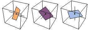
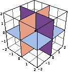
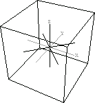
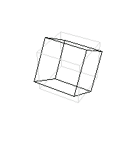
Using the functions ShowPlane from Structural Mechanics and DisplayTogetherArray from the Mathematica 4 Standard Add-on Packages, you can illustrate three perpendicular planes.
In[1]:=
In[2]:=DisplayTogetherArray[{ShowPlane[{1,0,0}],ShowPlane[{0,1,0}],ShowPlane[{0,0,1}]}];
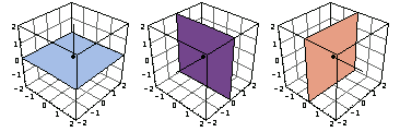
By using the function PrincipalPlane, you specify the origin of the direction vector, a scaling factor, and its direction.


First set some optional values to select a default font, frame the plot with a box, display grids on certain faces of the frame box, set the plot range, determine a viewpoint, and include the axes in the plot.
In[3]:=
Out[3]=
In[4]:=opts={Boxed->True,
FaceGrids->{{-1,0,0},{0,1,0},{0,0,-1}},
PlotRange->2{{-1,1},{-1,1},{-1,1}},
ViewPoint->{2.062,-2.275,2.052},
Axes->True};
Here are the same planes with these options set. If you choose the scaling factor 4, the plane surfaces completely partition the plot box.
In[5]:=plns=DisplayTogetherArray[
Graphics3D[PrincipalPlane[{0,0,0},{0,0,1},4],opts],
Graphics3D[PrincipalPlane[{0,0,0},{0,1,0},4],opts],
Graphics3D[PrincipalPlane[{0,0,0},{1,0,0},4],opts]];
Display these planes plns in a single plot with the DisplayTogether function from Graphics`Graphics` from the Mathematica 4 Standard Add-on Packages.
In[6]:=DisplayTogether[
Graphics3D[PrincipalPlane[{0,0,0},{0,0,1},4],opts],
Graphics3D[PrincipalPlane[{0,0,0},{0,1,0},4],opts],
Graphics3D[PrincipalPlane[{0,0,0},{1,0,0},4],opts]];
There are various ways to represent a stress tensor in Structural Mechanics. Now represent the stress components using the capital letter S and include the direction of a stress component as a subscript.
As described in Chapter 7, the StressComponents function generates the symbols representing the independent stress components in indicial notation.
In[7]:=strs=StressComponents[ , Cartesian[x,y,z],Notation-> Indicial] , Cartesian[x,y,z],Notation-> Indicial]
Out[7]=
This is a vector representation of the symmetric stress tensor. Use the function VectorToTensor to convert this form into a symmetric tensor representation of a stress state at a point.


In[8]:=tns=VectorToTensor[strs]
Out[8]=
In[9]:=MatrixForm[tns]
Out[9]//MatrixForm=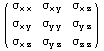
In addition to this indicial notation, here you use a functional notation for the stress components.
In[10]:=VectorToTensor[StressComponents[, Cartesian[x,y,z]]]
Out[10]=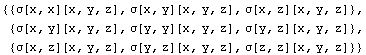
In[11]:=MatrixForm[%]
Out[11]//MatrixForm=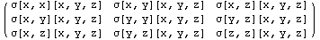
6.3 Principal Stresses and Directions
When the normal vector of a surface and the stress vector acting on that surface are colinear, the direction of the normal vector is called a principal stress direction. The magnitude of the stress vector on the surface is called the principal stress value. You use the function PrincipalStresses to calculate the principal stresses from the stress state at a point.
In the case where the values of all shear stresses are zero, the principal stresses are the normal stresses.
In[12]:=
Out[12]=
Similarly, you use the function PrincipalStressDirections to determine the directions of the principal stress components.


The principal stress directions are the unit vectors of the coordinate system in the case where no shear stress component is present.
In[13]:=
Out[13]=
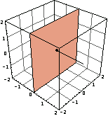
Visualize the first plane in the previously introduced graphics object plns, which orginated at the origin of the coordinate system.
In[14]:=Show[Graphics3D[PrincipalPlane[{0,0,0},{1,0,0},4]],opts];
Compute the principal stresses with a nonzero shear stress value for  . .
In[15]:=
Out[15]=
Note that the principal stress in the z-direction remains unchanged since the shear stress is applied in the x-y plane only. Now compute the principal stress directions for this stress tensor.
In[16]:=
Out[16]=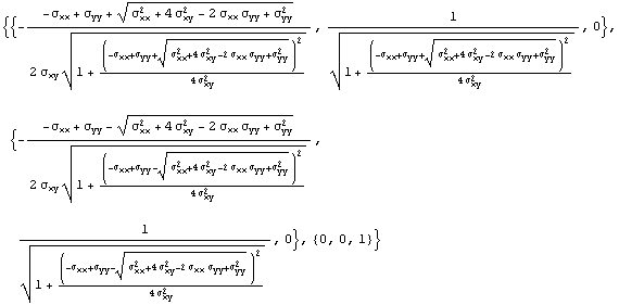
As expected, since the  components are zero, the positive direction of the z coordinate, {0, 0, 1} remains as a principal stress direction. components are zero, the positive direction of the z coordinate, {0, 0, 1} remains as a principal stress direction.
The function PrincipalStressDirectionsPlot plots the directions of principal stresses.

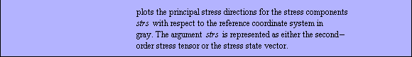
Show that the principal stress direction in the z-direction remains unchanged in the stress state  . Here the gray coordinates represent the reference coordinate system. . Here the gray coordinates represent the reference coordinate system.
In[17]:=PrincipalStressDirectionsPlot[{1,1,1,.5,0,0}];
PrincipalPlane graphics objects allow you to visualize these planes. First, compute the normal directions of the principal plane.
In[18]:={d1,d2,d3}=PrincipalStressDirections[{1,1,1,1/2,0,0}]
Out[18]=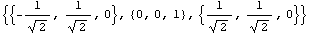
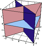
Here are the principal stress planes of this stress state.
In[19]:=planes=DisplayTogether[
Graphics3D[PrincipalPlane[{0,0,0},d1,5],opts],
Graphics3D[PrincipalPlane[{0,0,0},d2,5],opts],
Graphics3D[PrincipalPlane[{0,0,0},d3,5],opts],
ViewPoint->{0.947,-2.830,1.595}];
You determine the principal stresses by calculating the stress state at the directions  , ,  , ,  }. }.
In[20]:=
In[21]:=(newstr={d1,d2,d3}.tns.Transpose[{d1,d2,d3}])//MatrixForm
Out[21]//MatrixForm=
Equivalently, the function PrincipalStresses calculates the same values for a stress state.
In[22]:=PrincipalStresses[{1, 1, 1, 1/2, 0, 0}]
Out[22]=
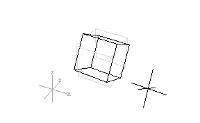
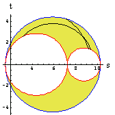
Another way to visualize these planes is to draw a picture of a rotated cube on whose surfaces the principal stresses are realized. You use the function UnitCubePlot for this purpose.
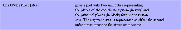
In[23]:=cube=UnitCubePlot[{5,4,7,0.01,0.03,2.91}];
The function PrincipalStressDirectionsPlot displays the principal stress direction in a different way.
In[24]:=dirs= PrincipalStressDirectionsPlot[{5,4,7,.01,.03,2.91}];
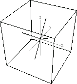
You extract the reference coordinate system from this graphics object dirs. Here you can generate a separate graphics object representing these directions.
In[25]:=
Similarly, you can also exact the principal stress directions from the same graphics object dirs.
In[26]:=p1=Graphics3D[dirs[[1,2]],Boxed->False];
Depicting these three figures cube,  , and , and  together provides a clear three-dimensional picture of the principal stress directions. You can arrange the relative positions of these graphics objects using the Mathematica graphics object Rectangle. together provides a clear three-dimensional picture of the principal stress directions. You can arrange the relative positions of these graphics objects using the Mathematica graphics object Rectangle.
In[27]:=Show[Graphics[{Rectangle[{0,0},{1,1},p0],
Rectangle[{0,0},{2,2},cube],
Rectangle[{1,0},{2,1},p1]
}]];
Calculate the stress invariants of a stress tensor with the function StressInvariants.
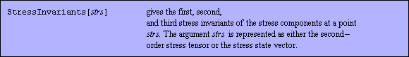
This calculates the stress invariants for a principal stress state.
In[28]:=
Out[28]=
If you add a shear term  , you can see how this shear stress affects the values of stress invariants. , you can see how this shear stress affects the values of stress invariants.
In[29]:=
Out[29]=
6.4 Maximum Shear Stresses and Directions
On a surface element in a continuum, you can always express the stress vector in terms of one normal component and one tangential component. A certain orientation of the surface element can show that maximum shear stresses are realized. This section considers the maximum shear stresses and their directions for a given stress state. First, consider the function MaximumShearStresses.

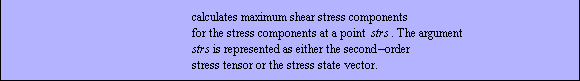
In[30]:=
Out[30]=
The expressions for the maximum shear stress components become complicated when you include the xy stress component in the stress tensor.
In[31]:=
Out[31]=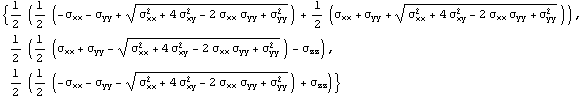
Similar to the function PrincipalStressDirections, you use the function MaximumShearDirections to compute the values of the maximum shear direction for a given stress state at a point.

In the principal stress directions, the shear components of the stress vector vanish. Thus, the shear stresses are zero in these directions.
Compute the maximum shear stresses for the stress vector {1, 2, 3, 0, 0, 0}.
In[32]:=MaximumShearStresses[{1,2,3,0,0,0}]
Out[32]=
The directions in which these values for the maximum shear stresses are realized are of practical interest. Calculate the maximum shear directions using the function MaximumShearDirections.
In[33]:=MaximumShearDirections[{1,2,3,0,0,0}]
Out[33]=
From this output, the maximum stress value is -1, and it acts on the plane whose normal vector is {1/ , 0, 1/ , 0, 1/ }. }.
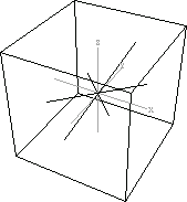
As in principal stress directions, you have the function MaximumShearDirectionsPlot to visualize the maximum shear stress direction for a given stress state.

This shows the maximum shear directions for the stress vector {1, 1, 1, 0.1, 0, 0}.
In[34]:=MaximumShearDirectionsPlot[{1,1,1,0.1,0,0}];
6.5 Mohr's Circles
Mohr's circles provide a planar representation of a three-dimensional stress state. Using Mohr's circles, you can calculate the stress state in a given direction graphically. The technique has been in use for over 100 years. Although current computer technology makes calculation of stress states easier, Structural Mechanics includes the method for its instructional and historical importance.
The function MohrsCircles generates the Mohr's circles for a given stress state.
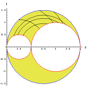
The gray areas in the Mohr's circles represent the stress states that can be realized by changing the orientation of the coordinate system for a given stress state. Here generate the Mohr's circles for the stress vector {1, 2, 4, 0, 0, 0}. The x axis (labeled with ) is the normal stress component, and the y axis (labeled with  ) is the tangent (shear) component. ) is the tangent (shear) component.
Compute the traction in a plane for which the normal vector is given by using a graphical method based on the technique used in Mohr's circles. The function MohrsCirclesTractions generates a pair of arches.


The crossing point of these two curves from MohrsCirclesTractions gives the normal and tangential components of the stress on the surface element whose direction is  , ,  , ,  ). ).
In[35]:=
In[36]:=p2=MohrsCirclesTraction[{1,2,4,0,0,0},{1,2,1}];
In[37]:=p3=MohrsCirclesTraction[{1,2,4,0,0,0},{1,2,3}];
In[38]:=
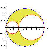
The approximate normal and tangential components for this state are {3.205263, 1.07034}. You can find the instructions for reading coordinates of a point on a two-dimensional plot by choosing the menu item Get Graphics Coordinates from the Input menu on the tool bar.
Superimpose the Mohr's circles for this stress state and the traction curves to illustrate where the crossing point of the two curves is located in the circle plot.
In[39]:=Show[p4,p1,p2,p3,PlotRange->All];
The function NormalShearStresses calculates the normal stress and shear components for given principal stresses and direction.


Here use exact values for the stress state vector {1, 2, 4} and their direction vector.
In[40]:=NormalShearStresses[{1,2,4},{1,2,3}/Sqrt[1+4+9] ]
Out[40]=
As expected, this result is exact. In order to compare it with the graphical result obtained using MohrsCirclesTraction earlier, {3.205263, 1.07034}, calculate the numerical values for this result using the function N.
In[41]:=N[%]
Out[41]=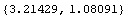
Now consider a more complicated example with shear stresses present.
In[42]:=strs={10.0,2.0,7.0,1.0,0.5,1.5}
Out[42]=
This is the stress state in tensor form.
In[43]:=VectorToTensor[strs]//MatrixForm
Out[43]//MatrixForm=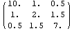
Produce the Mohr's circles for this stress state.
In[44]:=p1=MohrsCircles[strs,PlotRange->All];
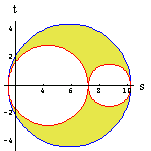
Graphically compute the normal stress and shear components in the direction (1, 2, 3).
In[45]:=p2=MohrsCirclesTraction[strs,{1,2,3}/Sqrt[14] ];
You can also compute these values by using NormalShearStresses. First compute the principal stresses.
In[46]:=pss=PrincipalStresses[strs]
Out[46]=
Calculate the normal and tangent components of the stresses in this direction.
In[47]:=NormalShearStresses[Sort[pss],{1,2,3}/Sqrt[1+4+9] ]
Out[47]=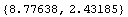
As shown in the previous Mohr's circles examples, you can graphically compute the principal stresses for this stress state with PrincipalStresses.
In[48]:=Show[p1,p2,PlotRange->All,AspectRatio->1];
Using the functions PrincipalStresses and NormalShearStresses, you compute the normal and tangential components for a given stress state. Now, consider the inverse problem; namely, the directions are computed from given principal stresses and the normal and shear stress components. Use the function NormalShearDirections to calculate the direction cosines of the plane in which a given normal stress and shear stresses are realized from the principal stress components.


Now compute the direction in which the given normal and shear components are {8.7, 2.4} for the principal stress values {10.275, 7.22, 1.50}.
In[49]:=nsd=NormalShearDirections[{10.275, 7.22, 1.50},{8.7,2.4}]
Out[49]=
This is the plane on which these values of the normal stress and shear stresses are realized.
In[50]:=Show[Graphics3D[PrincipalPlane[{0,0,0},nsd,5]],opts];
You can verify these values using the function NormalShearStresses.
In[51]:=NormalShearStresses[{10.275, 7.22, 1.50},nsd]
Out[51]=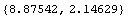
6.6 Failure Theories
This section uses the functionality in Structural Mechanics to consider three fundamental failure criteria:
 maximum normal stress theory maximum normal stress theory
maximum shear stress theory
distortion energy theory
6.6.1 The Maximum Normal Stress Theory
This simple theory is included only for its historical interest. Its predictions sometimes result in unsafe designs, and they do not agree with experimental data (e.g., the torsional analysis of bars). Thus, it is not recommended for use in modern designs. The maximum normal stress theory states that material failure occurs whenever the largest principal stress equals the strength of the material.
According to this theory, for the principal stresses,  , when the criterion of failure is the yielding stress, the failure occurs whenever , when the criterion of failure is the yielding stress, the failure occurs whenever  is equal to the tensile yield strength, or is equal to the tensile yield strength, or  is equal to the negative value of the compressive yield strength. The yielding failure criterion was used mostly for ductile materials. is equal to the negative value of the compressive yield strength. The yielding failure criterion was used mostly for ductile materials.
For brittle materials, the ultimate strength is used as the criterion of failure, and this theory predicts that the failure occurs whenever  is equal to the ultimate tensile strength, or is equal to the ultimate tensile strength, or  is equal to the negative value of the ultimate compressive strength. The following example demonstrates how the functions introduced in this chapter can be adopted in a design problem. is equal to the negative value of the ultimate compressive strength. The following example demonstrates how the functions introduced in this chapter can be adopted in a design problem.
Assume that the stress analysis results in a stress tensor (in MPa) as follows.
In[52]:=VectorToTensor[{300,450,-300,10,50,x}]//MatrixForm
Out[52]//MatrixForm=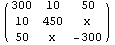
Here  is the stress component, which varies with the magnitude of the applied forces. Your task is to find the maximum value of x for a material whose tensile and compressive yield strengths are 600 MPa and 400 MPa, respectively. is the stress component, which varies with the magnitude of the applied forces. Your task is to find the maximum value of x for a material whose tensile and compressive yield strengths are 600 MPa and 400 MPa, respectively.
For x = 0, no failure occurs since the principal stresses components are between 600 MPa and -400 MPa.
In[53]:=PrincipalStresses[{300.,450.,-300.,10.,50.,0.}]
Out[53]=
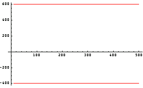
To solve this problem graphically, first mark the safety limits of the design.
In[54]:=limits=Plot[{600,-400},{x,10,500},PlotStyle->{RGBColor[1,0,0]}];
Plot the values of these three principal stresses by changing the value of x.
In[55]:=maxnormal=Plot[Evaluate[PrincipalStresses[{300,450,-300,10,50,x}]],{x,0,500}];
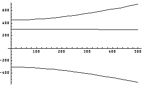
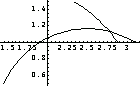
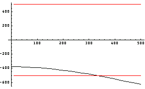
By superimposing these two plots, you can observe that two of the principal stresses cross the safety limits of the material at two points.
In[56]:=Show[{maxnormal,limits}];
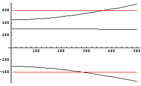
Thus,  = 286.98 MPa. = 286.98 MPa.
6.6.2 The Maximum Shear Stress Theory
The maximum shear stress theory is based on yielding, thus you can only use it for ductile materials. The theory states that yielding begins whenever the maximum shear stress in a mechanical element reaches the experimental maximum shear stress of the material of the element. According to this theory, the yield strength in shear is half of the normal yield strength.
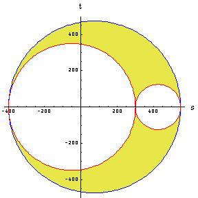
The maximum shear stress is ( - -  ) /2 where ) /2 where  are the principal stresses. This point is located at the uppermost point of Mohr's circles. are the principal stresses. This point is located at the uppermost point of Mohr's circles.
In[57]:=MohrsCircles[{300,450,-300,10,50,285}];
In[58]:={g3,g2,g1}=Sort[PrincipalStresses[{300.,450,-300,10,50,1}]]
Out[58]=
In[59]:=(g1-g3)/2
Out[59]=
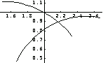
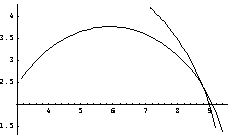
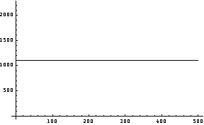
Plot the maximum shear stress as a function of x.
In[60]:=maxshear=Plot[gs=Evaluate[Sort[PrincipalStresses[{300.,450,-300,10,50,x}]]];.5(gs[[1]]-gs[[3]]),{x,0,500}];
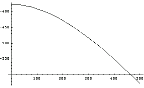
According to this theory, for a material with a yield strength of 1000 MPa, the limits of the yield strength in shear are -1000/2 = - 500 MPa and 1000/2 = 500 MPa.
In[61]:=limits=Plot[{1000/2,-1000/2},{x,10,500},PlotStyle->{RGBColor[1,0,0]}];
Superimposing this plot and the safety limit lines shows the location of the limit value for x.
In[62]:=Show[maxshear,limits];
The maximum shear theory is more conservative than the maximum normal stress theory. The results from the maximum shear theory are always on the "safe side." The coordinates of the approximate point where the yielding begins are {323.86, -498.98}:  = 323.86 MPa. = 323.86 MPa.
6.6.3 The Distortion Energy Theory
The distortion energy theory is also known as both the shear energy theory and the von Mises-Hencky theory. Like the maximum shear theory, this theory is only for ductile materials. The distortion energy theory produces the most conservative stress levels among the three methods considered in this chapter.
Using this theory, here is the criterion for the beginning of the yield.

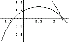
In this expression,  is the material yield strength, and is the material yield strength, and  , and , and  are the principal stresses. Solve this equality for are the principal stresses. Solve this equality for  and plot and plot  with respect to x as in the previous example for the same stress state. with respect to x as in the previous example for the same stress state.
In[63]:=maxshear=Plot[gs=Evaluate[Sort[PrincipalStresses[{300.,450,-300,10,50,x}]]];Sqrt[.5((gs[[1]]-gs[[2]])^2+(gs[[2]]-gs[[3]])^2+(gs[[3]]-gs[[1]])^2)],{x,0,500}];
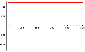
Draw the limiting lines for the same material used in the previous example.
In[64]:=limits=Plot[{1000,-1000},{x,10,500},
PlotStyle->RGBColor[1,0,0],
DisplayFunction->Identity
];
Superimposing these two plots shows for what value of x yielding begins.
In[65]:=Show[maxshear,limits];
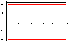
The coordinates for the approximate point where yielding begins are {416.27, 979.28}.
|