1.2.3 Covariance and Correlation FunctionsWe have defined the covariance and correlation functions of a stationary process in Section 1.2.2. We now illustrate how to obtain the covariance and the correlation functions of a given model using this package. The functions CovarianceFunction[model, h] and CorrelationFunction[model, h] give, respectively, the covariance and the correlation functions of the given model up to lag h, that is, { (0), (0),  (1), ... , (1), ... ,  (h)} (h)} and { (0), (0),  (1), ... , (1), ... ,  (h)} (h)}. The code for each function solves internally a set of difference equations obtained by multiplying both sides of ( 2.3) by Xt-k ( k=0, 1, ... ) and taking expectations. For mathematical details see Brockwell and Davis (1987), p. 92. We begin by considering the behavior of the covariance and correlation functions of AR models. Example 2.5 In Example 2.2 we derived the covariance and correlation functions of AR(1) model. Now we can obtain the same results using CovarianceFunction and CorrelationFunction. This calculates the covariance function of an AR(1) model up to lag 4. | Out[15]= |  |
These are the covariances at lags 0, 1, ..., 4. Note that the first entry in the output is  (0) (0), the variance of the series. To get the correlation function we need to divide the above result by its first entry  (0) (0). This can be done explicitly as follows. The correlation function of the AR(1) model is calculated up to lag 4. The expression %[[1]] represents the first element of the last output. | Out[16]= |  |
We may also obtain the correlation function directly. This gives the same correlation function up to lag 4. | Out[17]= |  |
Both CorrelationFunction and CovarianceFunction use the function StationaryQ to check the stationarity of the model before computing the correlation or covariance function. If the model is manifestly nonstationary, the covariance or the correlation is not calculated. When the model is not stationary, no correlation is calculated. | Out[18]= |  |
When symbolic coefficients are used, StationaryQ will not give True or False and the covariance and the correlation functions are calculated assuming the model is stationary, as we have seen in Example 2.5. Example 2.5 shows that the correlation function of an AR(1) process decays exponentially for a stationary model, and when  1<0 1<0 it oscillates between positive and negative values. In order to visualize the "shape" of the correlation function, we plot it as a function of the lag. Since the correlation function is a list of discrete values, we use the Mathematica function ListPlot to plot it. ListLinePlot could be used instead if a line plot through the values is desired. The output of CorrelationFunction or CovarianceFunction corresponds to lags 0, 1, 2, ..., while ListPlot assumes x coordinates of 1, 2, ... if x coordiantes are not explictly given. To match the lags with the correct correlation terms, we can either drop the first entry of the output of CorrelationFunction and plot { (1), (1),  (2), ... , (2), ... ,  (h)} (h)} using ListPlot, plot the output using ListPlot with an additional DataRange option, or input the correlation data to ListPlot in the form {{0,  (0)}, {1, (0)}, {1,  (1)}, ... , {h, (1)}, ... , {h,  (h)}} (h)}}. This form can be obtained by using Transpose. Here we recast the output of CorrelationFunction in the desired form. | Out[19]= |  |
The output can then be used as the argument of ListPlot. It is convenient to define a function that takes the output of CorrelationFunction and does the appropriate plot so the data does not need to be manually processed every time we plot the correlation function. We will choose to use the DataRange option to ListPlot and define the function plotcorr as follows. This defines plotcorr for plotting correlation functions. The first argument in plotcorr is the output of CorrelationFunction and the second is the usual set of options for ListPlot. Next we display the two typical forms of the correlation function of an AR(1) process, one for positive  1(=0.7) 1(=0.7) and one for negative  1(=-0.7) 1(=-0.7) using the function plotcorr. (Since the correlation function of a univariate time series is independent of the noise variance, we set  2=1 2=1.) This calculates the correlation function up to lag 10. The semicolon at the end of the command prevents the display of the output. This is the plot of the correlation function. | Out[22]= | 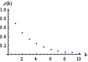 |
Note that if we do not need the correlation function for other purposes we can directly include the calculation of the correlation function inside the function plotcorr as shown below. This gives the plot of the correlation function for  1=-0.7 1=-0.7. | Out[23]= | 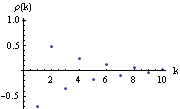 |
We have given the option AxesLabel -> {"k", " (k)"} (k)"} to label the axes. We can also specify other options of ListPlot. (To find out all the options of ListPlot use Options[ListPlot].) For example, if we want to join the points plotted, then the option Joined -> True should be given, and if we want to label the plot we use PlotLabel -> "label" as in the following example. Example 2.6 Plot the correlation function of the Yule, or AR(2), process: Xt=0.9Xt-1-0.8Xt-2+Zt. The correlation function of the given AR(2) process is plotted. For future re-display, we have called this graph g1 (see Example 5.1). | Out[24]= | 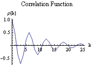 |
The way the correlation function decays is intimately related to the roots of  (x)=0 (x)=0. Complex roots give rise to oscillatory behavior of the correlation function as we observe in this example. For the explicit expression of the covariance function  (k) (k) in terms of the zeros of  (x) (x), see Brockwell and Davis (1987), Section 3.3. Next we study the behavior of MA models. Recall that the covariance function  (k) (k) of an ARMA process is calculated by multiplying both sides of ( 2.3) by Xt-k and computing expectations. Note that for an MA( q) process when k>q there is no overlap on the right-hand side of ( 2.3). Thus  (k)=0 (k)=0 (  (k)=0 (k)=0) for k>q. This is characteristic of the MA correlation function, and it is, in fact, often used to identify the order of an MA process, as we shall see in Section 1.5. Example 2.7 Find the correlation function up to lag 4 of an MA(2) process: Xt=Zt+ 1Zt-1+ 1Zt-1+ 2Zt-2 2Zt-2. This calculates the correlation function up to lag 4 of an MA(2) process. | Out[25]= |  |
We see that  (k)=0 (k)=0 for k>2. In fact, the correlation function of an MA model can be easily worked out analytically (see Brockwell and Davis (1977), p. 93). In particular, when an MA( q) model has equal  weights ( i.e.,  1= 1= 2=... = 2=... = q= q= ), the correlation function is given by  (0)=1 (0)=1,  (k)=0 (k)=0 for k>q, and  (k)=( (k)=( + + 2(q-k))/(1+ 2(q-k))/(1+ 2q) 2q) for 0<k≤q. In particular, when  = = 0=1 0=1, the correlation function is  (k)=(1+q-k)/(1+q) (k)=(1+q-k)/(1+q) for k≤q, a straight line with slope -1/(1+q). (For convenience, we define  0=1 0=1 so that the MA polynomial can be written as  (x)= (x)=  ixi ixi. Similarly we write the AR polynomial as  (x)= (x)=  ixi ixi with  0=1 0=1.) Example 2.8 Find the correlation function of an MA(8) model with equal  weights. This calculates the correlation function of an MA(8) model with equal  weights. | Out[26]= |  |
Note that we have avoided typing t1 eight times by using Table[t1, {8}] to generate the eight identical MA coefficients. To get the correlation function for  =1 =1 we can simply substitute t1=1 in the above expression using % /. t1 -> 1. This gives the correlation function for  =1 =1. | Out[27]= |  |
To emphasize the discrete nature of the correlation function some people prefer to plot the correlation function as discrete lines joining the points {i, 0} and {i,  (i)} (i)} for i=0, 1, ... , h. It is easy to implement this type of plot in Mathematica, via ListPlot with a Filling option. The function defined above is used to plot the correlation function of the MA(8) model with equal  weights. | Out[28]= | 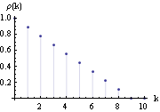 |
Example 2.9 The correlation function of a stationary ARMA( p, q) process in general decays exponentially. Here we plot the correlation function up to lag 10 of the ARMA(2, 2) model Xt-0.9Xt-1+0.3Xt-2=Zt+0.2Zt-1-1.2Zt-2 using the function plotcorr we defined earlier. The noise variance  2=1 2=1. This shows the correlation function of the ARMA(2, 2) model. | Out[29]= | 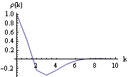 |
Using CorrelationFunction we can generate the correlation functions of different models; plotting the correlation functions enables us to develop intuition about different processes. The reader is urged to try a few examples. |