WSMLinearize["mmodel"]
gives a linearized state-space to the model "mmodel" at an equilibrium.
WSMLinearize["mmodel",{{{x1,x10},…},{{u1,u10},…}}]
linearizes at state values {x10,…} and input values {u10,…}.


WSMLinearize
WSMLinearize["mmodel"]
gives a linearized state-space to the model "mmodel" at an equilibrium.
WSMLinearize["mmodel",{{{x1,x10},…},{{u1,u10},…}}]
linearizes at state values {x10,…} and input values {u10,…}.
Details and Options
- WSMLinearize linearizes a continuous-time system designed in Wolfram System Modeler.
- WSMLinearize returns a StateSpaceModel object.
- WSMLinearize["mmodel",spec] allows the following symbolic values for spec:
-
"EquilibriumValues" uses WSMFindEquilibrium["mmodel"] "InitialValues" uses WSMModelData["mmodel","GroupedInitialValues"] - WSMLinearize["mmodel",vals,spec] uses spec to add missing values in vals.
- The default spec is taken to be "EquilibriumValues".
- The resulting StateSpaceModel has states xi, inputs uj, and outputs yk as defined in "mmodel".
- The list of states, inputs, and outputs can be found from WSMModelData["mmodel",spec]:
-
"StateVariables" state variables xi "InputVariables" input variables uj "OutputVariables" output variables yk - WSMLinearize reduces a system of DAEs to a system of ODEs and linearizes the resulting ODEs.
- A system of ODEs with state equations
 and output equations
  is linearized at a point
  and
and  .
. - The linearized system has state
 , input
  , and output
  , with state equations
  and output equation
  . The matrices are given by
  ,
,  ,
,  , and
, and  , all evaluated at
  and
and  .
. - The returned StateSpaceModel corresponds to the system
 ,
,  .
. - The shortest unique model name mmodel can be used where WSMNames["*.mmodel"] gives a unique match.
- The following options can be given:
-
Method "NumericDerivative" methods for linearization algorithm WSMProgressMonitor Automatic control display of progress - The option Method has the following possible settings:
-
"NumericDerivative" uses System Modeler linearization "SymbolicDerivative" uses StateSpaceModel linearization
Examples
open all close allBasic Examples (4)
Scope (13)
Model Types (5)
Limiting Cases (3)
Linearization Values (5)
Generalizations & Extensions (1)
Hide labels in the resulting StateSpaceModel:
Options (4)
Method (4)
By default, the "NumericDerivative" method is used:
The method "SymbolicDerivative" uses StateSpaceModel to linearize system equations:
Linearize symbolically, keeping some parameters symbolic:
Linearize symbolically, using a partially symbolic linearization point:
Applications (9)
Analyzing Linearized System (5)
Compare responses from a model and its linearization at an equilibrium point:
Linearize around the equilibrium point:
Compare the stationary output response with a nonlinear model:
Test the stability of a linearized system from eigenvalues of the system matrix:
Since there is an eigenvalue with a positive real part, the system is unstable:
Plotting the output response also indicates an unstable system:
Test the stability of a linearized system from poles of the transfer function:
Since there is a pole with a positive real part, the system is unstable:
Do a frequency analysis using a linear model:
By plotting ![]() for the linearized transfer function
for the linearized transfer function ![]() :
:
Verify the result using Fourier on simulated data:
Alternatively, the imaginary parts of the eigenvalues give the resonance peaks:
Linearization takes place at time 0:
Linearize with the switch connecting at time 0:
If the switch is not connected at time 0, the result is different:
Controller Design for Linearized System (4)
Design a lead-based controller for a DC motor based on its linearization:
Define a PI-lead controller transfer function:
Use selected parameters and close the loop with the PI-lead controller:
Design a controller using pole placement:
Compute the closed-loop state-space model:
Define state and input weight matrices:
Closed-loop state-space model:
Compute estimator gains and the estimator state-space model:
Properties & Relations (8)
Linearize around initial values using WSMModelData:
Linearize around equilibrium using WSMFindEquilibrium:
Compare responses from a model and its linearization at an equilibrium point:
Linearize around the equilibrium point:
Compare the stationary output response with a nonlinear model:
Compare responses from a model and its linearization at a non-equilibrium point:
Linearize around the given point:
Compare the stationary output response with a nonlinear model:
Compute the stationary output:
Use TransferFunctionModel to convert to a transfer function representation:
Use ToDiscreteTimeModel to discretize a linearized model:
Discretize using sample time ![]() :
:
The linearized state-space model is not unique:
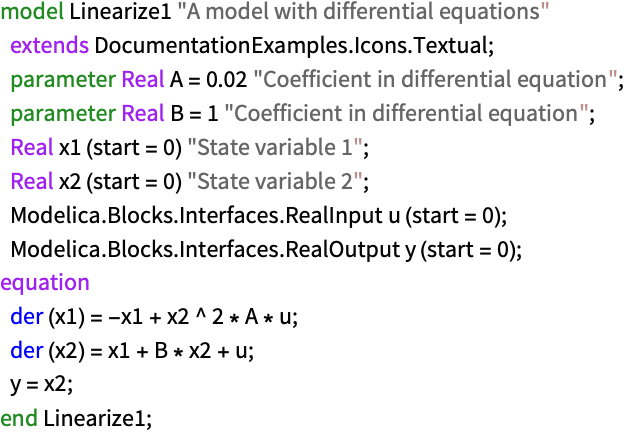
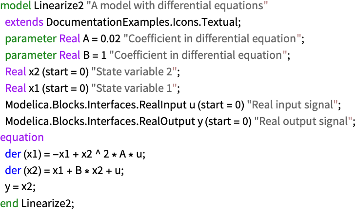
Change the order in which the variables x1 and x2 are declared:
The models are equivalent and have identical transfer functions:
StateSpaceModel can linearize systems of ordinary differential equations:
Using approximate numeric parameter values:
Using System Modeler to linearize a model of the same system:

