

EstimatedVariogramModel
EstimatedVariogramModel[{loc1val1,loc2val2,…}]
estimates the best variogram function from values vali given at locations loci.
EstimatedVariogramModel[{loc1,loc2,…}{val1,val2,…}]
generates the same result.
EstimatedVariogramModel[…,"model"]
estimates the best parameters of the variogram function specified by "model".
EstimatedVariogramModel[…,{"model",params}]
estimates the non-numeric parameters in params.
Details and Options
- Variogram model is also known as variogram and semivariogram.
- EstimatedVariogramModel fits a model to the spatial field data and returns a VariogramModel.
- VariogramModel is typically used as a local model of spatial dependence when predicting values of a spatial field, as in SpatialEstimate.
- The variogram
 for a spatial process
  at locations
  and
and  is given by
  . It is a measure of how quickly the process varies spatially.
 - When a process is weakly stationary, then the variogram depends only the difference of locations, i.e.
 . And when the process is isotropic, it only depends on the distance between locations
 ![gamma(TemplateBox[{{{p, _, 1}, -, {p, _, 2}}}, Norm])](Files/EstimatedVariogramModel.en/8.png "gamma(TemplateBox[{{{p, _, 1}, -, {p, _, 2}}}, Norm])") .
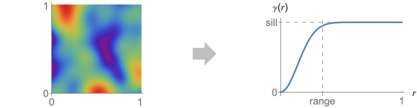
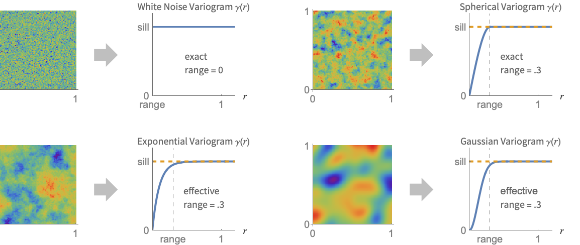
. - Typical examples of spatial field data that is stationary and isotropic together with the corresponding variogram.
- With automatic settings, this is all that is needed, but if you want to provide detailed control over the variogram model there are further aspects to understand. The two main issues are the range and level of smoothing.
- The range for the variogram indicates how far the dependence on nearby points extends. A larger range variogram will correspond to a slower varying field.
-
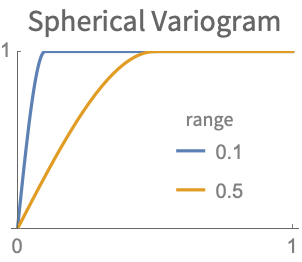

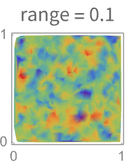
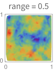
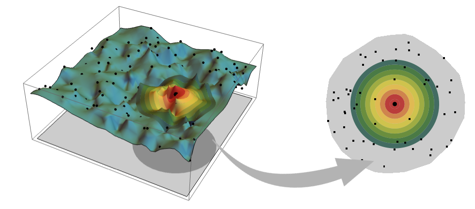
- The range of the variogram controls the distance at which points influence the range of prediction of values in SpatialEstimate.
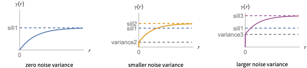
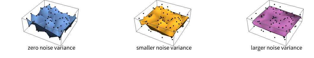
- The smoothness of the prediction is affected by the so-called spatial noise variance of the variogram, which is the value at the origin. It corresponds to adding a white noise model, e.g. measurement errors or true discontinuities in data such as a gold nugget.
- The size of the spatial noise variance controls the level of smoothing of values in SpatialEstimate. In particular, with a nonzero noise variance, the resulting surface will not interpolate the given values but instead approximate them.
- The locations loci can have the forms:
-
{p1,…,pd} geometrical locations GeoPosition[…],GeoPositionENU[…],… geographical locations - The values vali can have the forms:
-
ci scalar value Quantity[ci,"unit"] scalar quantity - The models need to satisfy consistency conditions to be a valid spatial variogram. It must be a non-negative function and satisfy the conditionally negative definite condition
![sum_(i=1)^nsum_(j=1)^nw_i w_j gamma(TemplateBox[{{{p, _, i}, -, {p, _, j}}}, Norm])<=0](Files/EstimatedVariogramModel.en/17.png "sum_(i=1)^nsum_(j=1)^nw_i w_j gamma(TemplateBox[{{{p, _, i}, -, {p, _, j}}}, Norm])<=0") for all weights wi such that
for all weights wi such that  and locations pi. The valid model families can be grouped into tables with similar features, and these are enumerated in VariogramModel.
 - The following options can be given:
-
SpatialNoiseLevel Automatic specify the noise variance in the model SpatialTrendFunction Automatic specify the global trend model
Examples
open all close allBasic Examples (2)
Estimate a variogram model for concentrations of zinc in soil:
locs = {...};
zinc = {...};PointValuePlot[locs -> zinc, ColorFunction -> "Rainbow"]Estimate exponential variogram model:
vf = EstimatedVariogramModel[locs -> zinc, "Exponential"]Extract the sill and range information:
{vf["Sill"], vf["Range"]}vf[120]vf["Visualization"]Estimate a white noise variogram model for random data:
locs = RandomPoint[Disk[], n = 300];
values = RandomReal[1, n];PointValuePlot[locs -> values]Estimate white noise variogram model:
ev = EstimatedVariogramModel[locs -> values, "WhiteNoise"]Plot[ev["Function"][z], {z, 0, 1}, PlotRange -> All]Scope (2)
Estimate variogram model for geographical data:
locs = GeoPosition[{{25.5, -124.5}, {25.5, -123.5}, {25.5, -122.5}, {25.5, -121.5}, {25.5, -120.5},
  {25.5, -112.5}, {25.5, -111.5}, {25.5, -110.5}, {25.5, -109.5}, {25.5, -108.5}, {25.5, -107.5},
  {25.5, -106.5}, {25.5, -105.5}, {25.5, -104.5}, {25.5 ... 8.5, -87.5}, {48.5, -86.5},
  {48.5, -85.5}, {48.5, -84.5}, {48.5, -83.5}, {48.5, -82.5}, {48.5, -81.5}, {48.5, -80.5},
  {48.5, -79.5}, {48.5, -78.5}, {48.5, -72.5}, {48.5, -71.5}, {48.5, -70.5}, {48.5, -69.5},
{48.5, -68.5}, {48.5, -67.5}}];ozone = {...};PointValuePlot[locs -> ozone, ColorFunction -> "Rainbow"]Fit a few models with slow initial variation:
models = {"Cubic", "Spherical", "Gaussian", "Matern"};vars = Map[EstimatedVariogramModel[locs -> ozone, #]&, models]Visualize the fit of variogram models to the binned variogram of the data:
Grid[Partition[MapThread[#1["Visualization", PlotLabel -> #2]&, {vars, models}], 2]]Estimate a variogram model from a binned variogram:
locations = {...};
vals = {...};bv = BinnedVariogramList[locations -> vals]ListPlot[bv]var = EstimatedVariogramModel[bv, "Power"]var["Visualization"]Options (3)
SpatialNoiseLevel (1)
Specify noise level using SpatialNoiseLevel:
SeedRandom["noise"];
locs = RandomPoint[Disk[], 200];
values = Exp[-Total /@ locs] + RandomReal[.5, 200];PointValuePlot[locs -> values, ColorFunction -> "Rainbow"]Estimate variogram model assuming zero noise level:
var0 = EstimatedVariogramModel[locs -> values, SpatialNoiseLevel -> 0]var0["Visualization"]Estimate variogram model assuming positive noise level:
var1 = EstimatedVariogramModel[locs -> values, SpatialNoiseLevel -> .01]var1["Visualization"]{var0["Parameters"], var1["Parameters"]}SpatialTrendFunction (2)
Specify trend function using SpatialTrendFunction:
SeedRandom["trend"];
locs = RandomPoint[Disk[], 200];
values = Exp[-Total /@ locs] + RandomReal[1, 200];PointValuePlot[locs -> values, ColorFunction -> "Rainbow"]Estimate variogram model assuming constant trend:
var0 = EstimatedVariogramModel[locs -> values, SpatialTrendFunction -> 0]var0["Visualization"]Estimate variogram model assuming linear trend:
var1 = EstimatedVariogramModel[locs -> values, SpatialTrendFunction -> 1]var1["Visualization"]{var0["Parameters"], var1["Parameters"]}Look at data with a linear trend:
BlockRandom[
SeedRandom["bvaiubvai"];
locs = RandomReal[1, {m = 10 ^ 3, 2}];
vals = 1 + locs . {2, 3} + RandomReal[.1, m];
]
Without detrending, the variogram is well fit by an unbounded model:
vf = EstimatedVariogramModel[locs -> vals, "Power", SpatialTrendFunction -> None]vf["Visualization"]Removing the large scale trend gives us a better idea of the micro scale variation:
vf2 = EstimatedVariogramModel[locs -> vals, "WhiteNoise", SpatialTrendFunction -> 1]vf2["Visualization"]Applications (2)
Estimate a variogram model for SpatialPointData:
data = ResourceData["Sample Data: Wheat Yield"]PointValuePlot[data, ColorFunction -> "Rainbow"]Compute the BinnedVariogramList to get an idea of which model family to choose:
bv = BinnedVariogramList[data]ListPlot[bv]Fit a few asymptotic variogram models:
models = {"Exponential", "Gaussian", "Matern", "PoweredExponential"};vars = Map[EstimatedVariogramModel[data, #]&, models]Visualize the fit of the variogram models to the binned variogram of the data:
Grid[Partition[MapThread[#1["Visualization", PlotLabel -> #2]&, {vars, models}], 2]]Out of the four models, Matern fits best and could be used for spatial estimation:
sef = SpatialEstimate[data, VariogramFunction -> vars[[3]]]sef["Visualization"]Use fit residuals to choose the best variogram model:
data = ResourceData["Sample Data: Wheat Yield"];PointValuePlot[data, ColorFunction -> "Rainbow"]models = {"Linear", "Cubic", "Matern", "Power"};vars = Map[EstimatedVariogramModel[data, #, SpatialTrendFunction -> 2]&, models];Compute the weighted sum of residuals from the fit:
residuals = Table[var["WeightedSumOfResiduals"], {var, vars}]Visualize the fit of variogram models to the binned variogram of the data:
Grid[Partition[MapThread[#1["Visualization", PlotRange -> {{0, 30}, All}, PlotLabel -> Column[{"Model: " <> #2, "Weighted Sum Of Residuals: " <> ToString@#3}]]&, {vars, models, residuals}], 2]]Choose the model with the smallest weighted sum of residuals and use it to compute spatial estimate:
best = First@Extract[models, Position[residuals, Min[residuals]]]sef = SpatialEstimate[data, VariogramFunction -> best]sef["Visualization"]Possible Issues (1)
Text
Wolfram Research (2021), EstimatedVariogramModel, Wolfram Language function, https://reference.wolfram.com/language/ref/EstimatedVariogramModel.html.
CMS
Wolfram Language. 2021. "EstimatedVariogramModel." Wolfram Language & System Documentation Center. Wolfram Research. https://reference.wolfram.com/language/ref/EstimatedVariogramModel.html.
APA
Wolfram Language. (2021). EstimatedVariogramModel. Wolfram Language & System Documentation Center. Retrieved from https://reference.wolfram.com/language/ref/EstimatedVariogramModel.html