


ListVectorDensityPlot
ListVectorDensityPlot[varr]
generates a vector density plot from an array varr of vector and scalar field values {{vxij,vyij},rij}.
ListVectorDensityPlot[{{{x1,y1},{{vx1,vy1},r1}},…}]
generates a vector density plot from vector and scalar field values {{vxi,vyi},ri} given at specified points {xi,yi}.
ListVectorDensityPlot[{data1,data2,…}]
plots data for several vector and scalar fields.
Details and Options
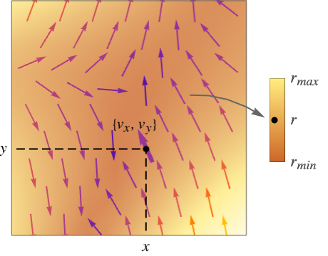
- ListVectorDensityPlot generates a vector plot of the vector field, superimposed on a background density plot of the scalar field.
- ListVectorDensityPlot displays a vector field by drawing arrows normalized to a fixed length. The arrows are colored by default according to the magnitude
 of the vector field. The vectors are drawn over a density plot of the scalar field r.
 - The magnitude
 of the vector field is used for the scalar field r by default.
 - The plot visualizes the set
 , where
  is the region for which
  is defined.
 - ListVectorDensityPlot interpolates the data into vector function
 and scalar function
  .
. - For regular data, the vector field
 has value varr〚i,j,1〛 and the scalar field has value varr〚i,j,2〛 at
  .
. - For irregular data, the vector field
 has value {vxi,vyi} and the scalar field has value riat
  .
. - If no scalar field values are given, they are taken to be the norm of the vector field.
- ListVectorDensityPlot[varr] arranges successive rows of varr up the page, and successive columns across.
- ListVectorDensityPlot by default interpolates the data given and plots vectors for the vector field at a regular grid of positions.
- With the setting VectorPoints->All, ListVectorDensityPlot instead shows vectors associated with the particular vector field data points given.
- ListVectorDensityPlot has the same options as Graphics, with the following additions and changes: [List of all options]
-
AspectRatio 1 ratio of height to width BoundaryStyle None how to draw RegionFunction boundaries BoxRatios Automatic effective 3D box ratios for simulated lighting ClippingStyle Automatic how to display arrows outside the vector range ColorFunction Automatic how to color background densities ColorFunctionScaling True whether to scale arguments to ColorFunction DataRange Automatic the range of x and y values to assume for data EvaluationMonitor None expression to evaluate at every function evaluation Frame True whether to draw a frame around the plot FrameTicks Automatic frame tick marks LightingAngle None effective angle for simulated lighting MaxRecursion Automatic the maximum number of recursive subdivisions allowed for the scalar field Mesh None how many mesh lines to draw in the background MeshFunctions {#5&} how to determine the placement of mesh lines MeshShading None how to shade regions between mesh lines MeshStyle Automatic the style of mesh lines Method Automatic methods to use for the plot PerformanceGoal $PerformanceGoal aspects of performance to try to optimize PlotLegends None legends for color gradients PlotRange {Full,Full} range of x, y values to include PlotRangePadding Automatic how much to pad the range of values PlotTheme $PlotTheme overall theme for the plot RegionFunction (True&) determine what region to include ScalingFunctions None how to scale individual coordinates VectorColorFunction Automatic how to color vectors VectorColorFunctionScaling True whether to scale the arguments to VectorColorFunction VectorMarkers Automatic shape to use for vectors VectorPoints Automatic the number or placement of vectors to plot VectorRange Automatic range of vector lengths to show VectorScaling Automatic how to scale the sizes of arrows VectorSizes Automatic sizes of displayed arrows VectorStyle Automatic how to draw vectors WorkingPrecision MachinePrecision precision to use in internal computations - The arguments supplied to functions in MeshFunctions, RegionFunction, ColorFunction, and VectorColorFunction are x, y, vx, vy, r.
- The default setting MeshFunctions->{#5&} draws mesh lines for the scalar field r.
- Possible settings for ScalingFunctions are:
-
{sx,sy} scale x and y axes - Common built-in scaling functions s include:
-
"Log" 
log scale with automatic tick labeling "Log10" 
base-10 log scale with powers of 10 for ticks "SignedLog" 
log-like scale that includes 0 and negative numbers "Reverse" 
reverse the coordinate direction "Infinite" 
infinite scale
List of all options
Examples
open all close allBasic Examples (2)
Plot the vector field with its norm as a background interpolated from a specified set of vectors:
ListVectorDensityPlot[Table[{y, -x}, {x, -3, 3, 0.2}, {y, -3, 3, 0.2}]]Plot the vector field from data specifying coordinates and vectors:
data = Table[{{x, y}, {y, x - x ^ 3}}, {x, -1.5, 1.5, 0.2}, {y, -2, 2, 0.2}];ListVectorDensityPlot[data]Scope (20)
Sampling (9)
Plot streamlines for a regular collection of vectors, and give a data range for the domain:
ListVectorDensityPlot[Table[{y, -x}, {x, -3, 3, 0.2}, {y, -3, 3, 0.2}], DataRange -> {{-3, 3}, {-3, 3}}]Plot an irregular collection of vectors:
data = Table[{{x, y} = RandomReal[{-3, 3}, {2}], {y, -x}}, {200}];ListVectorDensityPlot[data]Show all of the specified field vectors:
ListVectorDensityPlot[data, VectorPoints -> All]Explicitly set the number of vectors in each direction:
ListVectorDensityPlot[data, VectorPoints -> {4, 7}]data = Table[{{x, y}, {{y, x - x ^ 3}, Abs[x]}}, {x, -1.5, 1.5, 0.2}, {y, -2, 2, 0.2}];ListVectorDensityPlot[data]Use an explicit scalar field on an irregular collection of vectors:
data = Table[{{x, y} = RandomReal[{-1.5, 1.5}, {2}], {{y, x - x ^ 3}, Abs[x]}}, {300}];ListVectorDensityPlot[data, VectorPoints -> All]Plot two vector fields with background based on the norm of the first:
data1 = Table[{{x, y} = RandomReal[{-3, 3}, {2}], {y, -x}}, {200}];
data2 = Table[{{x, y} = RandomReal[{-3, 3}, {2}], {y ^ 2, x - y}}, {150}];ListVectorDensityPlot[{data1, data2}, VectorPoints -> 10]Specify a list of points for showing field vectors:
ListVectorDensityPlot[Table[{y, -x}, {x, -3, 3, 0.2}, {y, -3, 3, 0.2}], DataRange -> {{-3, 3}, {-3, 3}}, VectorPoints -> RandomReal[{-3, 3}, {300, 2}]]Plot a vector field with specified vector densities:
data = Table[{y, -x}, {x, -2, 2, 0.2}, {y, -2, 2, 0.2}];Table[ListVectorDensityPlot[data, PlotLabel -> p, VectorPoints -> p], {p, {5, Coarse, Automatic, Fine}}]Plot the vectors that go through a set of seed points:
points = {{-1, -1}, {-1, 1}, {1, -1}, {1, 1}};
data = Table[{-1 - x ^ 2 + y, 1 + x - y ^ 2}, {x, -3, 3, 0.2}, {y, -3, 3, 0.2}];ListVectorDensityPlot[data, DataRange -> {{-3, 3}, {-3, 3}}, VectorPoints -> points, VectorSizes -> 2, Epilog -> {Red, PointSize[Medium], Point[points]}]Plot vectors over a specified region:
ListVectorDensityPlot[Table[{{x, y} = RandomReal[{-3, 3}, {2}], {y, -x}}, {200}], RegionFunction -> Function[{x, y, vx, vy, n}, x y < 1]]Presentation (11)
Plot a vector field with arrows scaled according to their magnitudes:
ListVectorDensityPlot[Table[{y, -x}, {x, -3, 3, 0.2}, {y, -3, 3, 0.2}], VectorScaling -> Automatic]Use a single color for the arrows:
ListVectorDensityPlot[Table[{y, -x}, {x, -3, 3, 0.2}, {y, -3, 3, 0.2}], VectorColorFunction -> None]Plot a vector field with arrows of specified size:
data = Table[{x, -y}, {x, -3, 3, 0.2}, {y, -3, 3, 0.2}];Table[ListVectorDensityPlot[data, VectorColorFunction -> Hue, PlotLabel -> s, VectorSizes -> s], {s, {Small, Medium, Large, 0.5}}]data = Table[{Sin[x], Cos[y]}, {x, -Pi, Pi, 0.2}, {y, -Pi, Pi, 0.2}];Table[ListVectorDensityPlot[data, PlotLabel -> s, VectorAspectRatio -> s], {s, {0.25, 0.5}}]Plot a vector field with the background and vectors colored according to the field magnitude:
VectorDensityPlot[{y, -x}, {x, -3, 3}, {y, -3, 3}, ColorFunction -> "Pastel", VectorColorFunction -> Hue]Set the style for multiple vector fields:
data1 = Table[{-1 - x ^ 2 + y, 1 + x - y ^ 2}, {x, -3, 3, 0.2}, {y, -3, 3, 0.2}];
data2 = Table[{-(1 + x - y ^ 2), -1 - x ^ 2 + y}, {x, -3, 3, 0.2}, {y, -3, 3, 0.2}];ListVectorDensityPlot[{data1, data2}, VectorPoints -> 8, VectorStyle -> {{Red, "Drop"}, {Blue, "Dart"}}, VectorColorFunction -> None]data = Table[{-1 - x ^ 2 + y, 1 + x - y ^ 2}, {x, -3, 3, 0.2}, {y, -3, 3, 0.2}];ListVectorDensityPlot[data, VectorPoints -> 8, VectorStyle -> Arrowheads[{{0.03, Automatic, Graphics[Circle[]]}}]]Use a named appearance to draw the vectors:
data = Table[{y, -x}, {x, -3, 3, 0.2}, {y, -3, 3, 0.2}];ListVectorDensityPlot[data, VectorMarkers -> "Drop"]ListVectorDensityPlot[data, VectorMarkers -> "Drop", VectorColorFunction -> None, VectorStyle -> Red]Use a legend for the color gradients:
data = Table[{-1 - x ^ 2 + y, 1 + x - y ^ 2}, {x, -3, 3, 0.2}, {y, -3, 3, 0.2}];ListVectorDensityPlot[data, VectorStyle -> Red, VectorColorFunction -> None, PlotLegends -> Automatic]Use a theme with detailed frame ticks and grid lines:
data = Table[{-1 - x ^ 2 + y, 1 + x - y ^ 2}, {x, -3, 3, 0.2}, {y, -3, 3, 0.2}];ListVectorDensityPlot[data, PlotTheme -> "Detailed"]Use a theme with a high-contrast color scheme and edge-fading rectangles:
data = Table[{-1 - x ^ 2 + y, 1 + x - y ^ 2}, {x, -3, 3, 0.2}, {y, -3, 3, 0.2}];ListVectorDensityPlot[data, PlotTheme -> "Marketing"]Reverse the direction of the y axis:
ListVectorDensityPlot[Flatten[Table[{{x, y}, {x, y - x}}, {x, -3, 3, 0.2}, {y, -3, 3, 0.2}], 1], ScalingFunctions -> {None, "Reverse"}]Options (87)
Background (1)
BoundaryStyle (2)
By default, region boundaries have no style:
data = Table[{Sin[x], Cos[y]}, {x, -3, 3, 0.2}, {y, -3, 3, 0.2}];ListVectorDensityPlot[data]Change the style of the boundary:
data = Table[{Sin[x], Cos[y]}, {x, -3, 3, 0.2}, {y, -3, 3, 0.2}];ListVectorDensityPlot[data, BoundaryStyle -> Directive[Thick, Black]]ColorFunction (6)
Color the field magnitude using Hue:
ListVectorDensityPlot[Table[{y, -x}, {x, -3, 3, 0.2}, {y, -3, 3, 0.2}], MaxRecursion -> 2, ColorFunction -> Hue]Color using Hue based on ![]() :
:
ListVectorDensityPlot[Table[{{y, -x}, Sin[x y]}, {x, -3, 3, 0.2}, {y, -3, 3, 0.2}], MaxRecursion -> 2, ColorFunction -> Hue]Use any named color gradient from ColorData:
ListVectorDensityPlot[Table[{-1 - x ^ 2 + y, 1 + x - y ^ 2}, {x, -3, 3, 0.2}, {y, -3, 3, 0.2}], ColorFunction -> "Pastel"]Use ColorData for predefined color gradients:
data = Table[{-1 - x ^ 2 + y, 1 + x - y ^ 2}, {x, -3, 3, 0.2}, {y, -3, 3, 0.2}];ListVectorDensityPlot[data, ColorFunction -> Function[{x, y, vx, vy, n}, ColorData["SolarColors"][x y]]]Specify a color function that blends two colors by the ![]() coordinate:
coordinate:
data = Table[{-1 - x ^ 2 + y, 1 + x - y ^ 2}, {x, -3, 3, 0.2}, {y, -3, 3, 0.2}];ListVectorDensityPlot[data, ColorFunction -> Function[{x, y, vx, vy, n}, Blend[{Green, Red}, x]]]Use ColorFunctionScaling->False to get unscaled values:
data = Table[{-1 - x ^ 2 + y, 1 + x - y ^ 2}, {x, -3, 3, 0.2}, {y, -3, 3, 0.2}];ListVectorDensityPlot[data, MaxRecursion -> 4, ColorFunctionScaling -> False, ColorFunction -> Function[{x, y, vx, vy, n}, ColorData[22][Round[n]]]]ColorFunctionScaling (4)
By default, scaled values are used:
data = Table[{y Cos[x y], x Cos[x y]}, {x, -3, 3, 0.2}, {y, -3, 3, 0.2}];ListVectorDensityPlot[data, MaxRecursion -> 2, ColorFunction -> GrayLevel]Use ColorFunctionScaling->False to get unscaled values:
data = Table[{y Cos[x y], x Cos[x y]}, {x, -3, 3, 0.2}, {y, -3, 3, 0.2}];ListVectorDensityPlot[data, MaxRecursion -> 4, ColorFunctionScaling -> False, ColorFunction -> Function[{x, y, vx, vy, n}, ColorData[22][Round[n]]]]Use unscaled coordinates in the ![]() direction and scaled coordinates in the
direction and scaled coordinates in the ![]() direction:
direction:
data = Table[{y Cos[x y], x Cos[x y]}, {x, -3, 3, 0.2}, {y, -3, 3, 0.2}];ListVectorDensityPlot[data, ColorFunctionScaling -> {False, True}, ColorFunction -> Function[{x, y, vx, vy, n}, Hue[x, y, 1]]]Explicitly specify the scaling for each color function argument:
data = Table[{y Cos[x y], x Cos[x y]}, {x, -3, 3, 0.2}, {y, -3, 3, 0.2}];ListVectorDensityPlot[data, MaxRecursion -> 3, ColorFunctionScaling -> {True, True, True, True, False}, ColorFunction -> Function[{x, y, vx, vy, n}, Hue[n, y, 1]]]DataRange (1)
By default, the data range is taken to be the index range of the data array:
data = Table[{y, -x}, {x, -3, 3, 0.2}, {y, -3, 3, 0.3}];
Dimensions[data]ListVectorDensityPlot[data]Specify the data range for the domain:
ListVectorDensityPlot[data, DataRange -> {{-3, 3}, {-3, 3}}]EvaluationMonitor (1)
MaxRecursion (1)
Mesh (5)
By default, no mesh lines are displayed:
ListVectorDensityPlot[Table[{-1 - x ^ 2 + y, 1 + x - y ^ 2}, {x, -3, 3, 0.2}, {y, -3, 3, 0.2}], Mesh -> None]Show the initial and final sampling meshes:
Table[ListVectorDensityPlot[Table[{-1 - x ^ 2 + y, 1 + x - y ^ 2}, {x, -3, 3, 0.2}, {y, -3, 3, 0.2}], PlotLabel -> m, Mesh -> m], {m, {Full, Automatic}}]Use a specific number of mesh lines:
ListVectorDensityPlot[Table[{-1 - x ^ 2 + y, 1 + x - y ^ 2}, {x, -3, 3, 0.2}, {y, -3, 3, 0.2}], Mesh -> 5]ListVectorDensityPlot[Table[{-1 - x ^ 2 + y, 1 + x - y ^ 2}, {x, -3, 3, 0.2}, {y, -3, 3, 0.2}], Mesh -> {{2, 4, 5}}]Use different styles for different mesh lines:
data = Table[{-1 - x ^ 2 + y, 1 + x - y ^ 2}, {x, -3, 3, 0.2}, {y, -3, 3, 0.2}];ListVectorDensityPlot[data, Mesh -> {{{2, Thick}, {4, Yellow}, {5, {Thick, Red, Dashed}}}}]MeshFunctions (3)
By default, mesh lines correspond to the magnitude of the field:
data = Table[{-1 - x ^ 2 + y, 1 + x - y ^ 2}, {x, -3, 3, 0.2}, {y, -3, 3, 0.2}];ListVectorDensityPlot[data, Mesh -> 5, MeshFunctions -> Function[{x, y, vx, vy, n}, n]]Use the ![]() value as the mesh function:
value as the mesh function:
data = Table[{-1 - x ^ 2 + y, 1 + x - y ^ 2}, {x, -3, 3, 0.2}, {y, -3, 3, 0.2}];ListVectorDensityPlot[data, Mesh -> 5, MeshFunctions -> Function[{x, y, vx, vy, n}, x]]Use mesh lines corresponding to fixed distances from the origin:
data = Table[{-1 - x ^ 2 + y, 1 + x - y ^ 2}, {x, -3, 3, 0.2}, {y, -3, 3, 0.2}];ListVectorDensityPlot[data, DataRange -> {{-3, 3}, {-3, 3}}, Mesh -> 5, MeshFunctions -> Function[{x, y, vx, vy, n}, Sqrt[x ^ 2 + y ^ 2]]]MeshShading (3)
Use None to remove regions:
data = Table[{-1 - x ^ 2 + y, 1 + x - y ^ 2}, {x, -3, 3, 0.2}, {y, -3, 3, 0.2}];ListVectorDensityPlot[data, Mesh -> 10, MeshShading -> {Red, None}]data = Table[{-1 - x ^ 2 + y, 1 + x - y ^ 2}, {x, -3, 3, 0.2}, {y, -3, 3, 0.2}];ListVectorDensityPlot[data, Mesh -> 10, MeshShading -> {Red, Yellow, Green, None}]Use indexed colors from ColorData cyclically:
data = Table[{-1 - x ^ 2 + y, 1 + x - y ^ 2}, {x, -3, 3, 0.2}, {y, -3, 3, 0.2}];ListVectorDensityPlot[data, Mesh -> 10, MeshShading -> ColorData[51, "ColorList"]]MeshStyle (1)
PerformanceGoal (2)
Generate a higher-quality plot:
ListVectorDensityPlot[Table[{-1 - x ^ 2 + y, 1 + x - y ^ 2}, {x, -3, 3, 0.2}, {y, -3, 3, 0.2}], PerformanceGoal -> "Quality"]Emphasize performance, possibly at the cost of quality:
ListVectorDensityPlot[Table[{-1 - x ^ 2 + y, 1 + x - y ^ 2}, {x, -3, 3, 0.2}, {y, -3, 3, 0.2}], PerformanceGoal -> "Speed"]PlotLegends (2)
Use legends for vector color gradients:
ListVectorDensityPlot[Table[{-1 - x ^ 2 + y, 1 + x - y ^ 2}, {x, -2, 2, .2}, {y, -2, 2, .2}], PlotLegends -> Automatic]Use Placed to put legends above the plot:
ListVectorDensityPlot[Table[{-1 - x ^ 2 + y, 1 + x - y ^ 2}, {x, -2, 2, .2}, {y, -2, 2, .2}], PlotLegends -> Placed[Automatic, Above]]PlotRange (7)
The full plot range is used by default:
ListVectorDensityPlot[Table[{-1 - x ^ 2 + y, 1 + x - y ^ 2}, {x, -3, 3, 0.2}, {y, -3, 3, 0.2}], PlotRange -> Full]Specify an explicit limit for both ![]() and
and ![]() ranges:
ranges:
ListVectorDensityPlot[Table[{-1 - x ^ 2 + y, 1 + x - y ^ 2}, {x, -3, 3, 0.2}, {y, -3, 3, 0.2}], DataRange -> {{-3, 3}, {-3, 3}}, PlotRange -> 2]ListVectorDensityPlot[Table[{-1 - x ^ 2 + y, 1 + x - y ^ 2}, {x, -3, 3, 0.2}, {y, -3, 3, 0.2}], DataRange -> {{-3, 3}, {-3, 3}}, PlotRange -> {{-1, 2}, Automatic}]Specify an explicit ![]() minimum range:
minimum range:
ListVectorDensityPlot[Table[{-1 - x ^ 2 + y, 1 + x - y ^ 2}, {x, -3, 3, 0.2}, {y, -3, 3, 0.2}], DataRange -> {{-3, 3}, {-3, 3}}, PlotRange -> {{0, Full}, Automatic}]ListVectorDensityPlot[Table[{-1 - x ^ 2 + y, 1 + x - y ^ 2}, {x, -3, 3, 0.2}, {y, -3, 3, 0.2}], DataRange -> {{-3, 3}, {-3, 3}}, PlotRange -> {Full, {0, 2}}]Specify an explicit ![]() maximum range:
maximum range:
ListVectorDensityPlot[Table[{-1 - x ^ 2 + y, 1 + x - y ^ 2}, {x, -3, 3, 0.2}, {y, -3, 3, 0.2}], DataRange -> {{-3, 3}, {-3, 3}}, PlotRange -> {Full, {Full, 5}}]ListVectorDensityPlot[Table[{-1 - x ^ 2 + y, 1 + x - y ^ 2}, {x, -3, 3, 0.2}, {y, -3, 3, 0.2}], DataRange -> {{-3, 3}, {-3, 3}}, PlotRange -> {{-2, 1.5}, {-1, 2}}]PlotTheme (2)
Use a theme with simple ticks and grid lines in a high-contrast color scheme:
ListVectorDensityPlot[Table[{-1 - x ^ 2 + y, 1 + x - y ^ 2}, {x, -3, 3, 0.2}, {y, -3, 3, 0.2}], DataRange -> {{-3, 3}, {-3, 3}}, PlotTheme -> "Business"]ListVectorDensityPlot[Table[{-1 - x ^ 2 + y, 1 + x - y ^ 2}, {x, -3, 3, 0.2}, {y, -3, 3, 0.2}], DataRange -> {{-3, 3}, {-3, 3}}, PlotTheme -> "Marketing"]RegionBoundaryStyle (4)
The boundaries of full rectangular regions are not shown:
data = Table[{Cos[x], y}, {x, -3, 3, 0.2}, {y, -3, 3, 0.2}];ListVectorDensityPlot[data, DataRange -> {{-3, 3}, {-3, 3}}]Show the region being plotted:
data = Table[{Cos[x], y}, {x, -3, 3, 0.2}, {y, -3, 3, 0.2}];ListVectorDensityPlot[data, DataRange -> {{-3, 3}, {-3, 3}}, RegionFunction -> Function[{x, y, vx, vy, n}, x^2 + y^2 ≤ 9]]Specify a style for the boundary:
data = Table[{Cos[x], y}, {x, -3, 3, 0.2}, {y, -3, 3, 0.2}];ListVectorDensityPlot[data, DataRange -> {{-3, 3}, {-3, 3}}, RegionFunction -> Function[{x, y, vx, vy, n}, x^2 + y^2 ≤ 9], RegionBoundaryStyle -> Directive[Thick, Magenta]]Specify a style for full rectangular regions:
data = Table[{Cos[x], y}, {x, -3, 3, 0.2}, {y, -3, 3, 0.2}];ListVectorDensityPlot[data, DataRange -> {{-3, 3}, {-3, 3}}, RegionBoundaryStyle -> Directive[Thick, Black]]RegionFunction (3)
Plot vectors only over certain quadrants:
data = Table[{-1 - x ^ 2 + y, 1 + x - y ^ 2}, {x, -3, 3, 0.2}, {y, -3, 3, 0.2}];ListVectorDensityPlot[data, DataRange -> {{-3, 3}, {-3, 3}}, RegionFunction -> Function[{x, y, vx, vy, n}, x y < 1]]Plot vectors only over regions where the field magnitude is above a given threshold:
data = Table[{-1 - x ^ 2 + y, 1 + x - y ^ 2}, {x, -3, 3, 0.2}, {y, -3, 3, 0.2}];ListVectorDensityPlot[data, DataRange -> {{-3, 3}, {-3, 3}}, RegionFunction -> Function[{x, y, vx, vy, n}, n > 6], MaxRecursion -> 1]Use any logical combination of conditions:
data = Table[{-1 - x ^ 2 + y, 1 + x - y ^ 2}, {x, -3, 3, 0.2}, {y, -3, 3, 0.2}];ListVectorDensityPlot[data, DataRange -> {{-3, 3}, {-3, 3}}, RegionFunction -> Function[{x, y, vx, vy, n}, 4 < n < 9 || n < 2], MaxRecursion -> 2]ScalingFunctions (3)
By default, linear scales are used:
ListVectorDensityPlot[Table[{y, x - y}, {x, -1, 1, 0.1}, {y, -1, 1, 0.1}]]Use a log scale in the y direction:
ListVectorDensityPlot[Table[{y, x - y}, {x, -1, 1, 0.1}, {y, -1, 1, 0.1}], ScalingFunctions -> {None, "Log"}]Reverse the direction of the y direction:
ListVectorDensityPlot[Table[{y, x - y}, {x, -1, 1, 0.1}, {y, -1, 1, 0.1}], ScalingFunctions -> {None, "Reverse"}]VectorAspectRatio (1)
Specify arrowhead size relative to the length of the arrow with VectorAspectRatio:
ListVectorDensityPlot[Table[{Sin[x], Cos[y]}, {x, -Pi, Pi, 0.2}, {y, -Pi, Pi, 0.2}], VectorAspectRatio -> 1 / 2]VectorColorFunction (4)
Color the vectors according to their norms:
data = Table[{y, -x}, {x, -3, 3, 0.2}, {y, -3, 3, 0.2}];ListVectorDensityPlot[data, VectorColorFunction -> Hue]Use any named color gradient from ColorData:
data = Table[{y, -x}, {x, -3, 3, 0.2}, {y, -3, 3, 0.2}];ListVectorDensityPlot[data, VectorColorFunction -> "Rainbow"]Color the vectors according to their ![]() values:
values:
data = Table[{y, -x}, {x, -3, 3, 0.2}, {y, -3, 3, 0.2}];ListVectorDensityPlot[data, VectorColorFunction -> Function[{x, y, vx, vy, n}, ColorData["ThermometerColors"][x]]]Use VectorColorFunctionScaling->False to get unscaled values:
data = Table[{y, -x}, {x, -3, 3, 0.2}, {y, -3, 3, 0.2}];ListVectorDensityPlot[data, VectorColorFunction -> Function[{x, y, vx, vy, n}, ColorData[31][Round[n]]], VectorColorFunctionScaling -> False]VectorColorFunctionScaling (4)
By default, scaled values are used:
ListVectorDensityPlot[Table[{y, -x}, {x, -3, 3, 0.2}, {y, -3, 3, 0.2}], VectorColorFunction -> Hue]Use VectorColorFunctionScaling->False to get unscaled values:
data = Table[{y, -x}, {x, -3, 3, 0.2}, {y, -3, 3, 0.2}];ListVectorDensityPlot[data, VectorColorFunction -> Function[{x, y, vx, vy, n}, ColorData[31][Round[n]]], VectorColorFunctionScaling -> False]Use unscaled coordinates in the ![]() direction and scaled coordinates in the
direction and scaled coordinates in the ![]() direction:
direction:
data = Table[{y, -x}, {x, 0, 1, 0.1}, {y, 0, 1, 0.1}];ListVectorDensityPlot[data, DataRange -> {{0, 2}, {0, 2}}, VectorColorFunction -> Function[{x, y, vx, vy, n}, Hue[x, y, 1]], VectorColorFunctionScaling -> {False, True}]Explicitly specify the scaling for each color function argument:
data = Table[{y, -x}, {x, 0, 1, 0.1}, {y, 0, 1, 0.1}];ListVectorDensityPlot[data, DataRange -> {{0, 2}, {0, 2}}, VectorColorFunction -> Function[{x, y, vx, vy, n}, Hue[n, y, 1]], VectorColorFunctionScaling -> {True, True, True, True, False}]VectorMarkers (10)
Vectors are drawn as arrows by default:
data = Table[{y, -x}, {x, -3, 3, 0.2}, {y, -3, 3, 0.2}];ListVectorDensityPlot[data]Use a named appearance to draw the vectors:
data = Table[{y, -x}, {x, -3, 3, 0.2}, {y, -3, 3, 0.2}];ListVectorDensityPlot[data, VectorMarkers -> "Drop"]Use different markers for different vector fields:
data1 = Table[{{x, y}, {y, -x}}, {x, -5, 5}, {y, -5, 5}];
data2 = Table[{{x, y}, {x, y}}, {x, -5, 5}, {y, -5, 5}];ListVectorDensityPlot[{data1, data2}, VectorMarkers -> {"Drop", "Dart"}]By default, markers are centered on vector points:
data = Table[{{x, y}, {y, -x}}, {x, -5, 5}, {y, -5, 5}];pts = Tuples[Range[-5, 5], 2];ListVectorDensityPlot[data, VectorMarkers -> "Arrow", VectorPoints -> pts, Epilog -> {Red, Point[pts]}]Start the vectors at the points:
ListVectorDensityPlot[data, VectorMarkers -> Placed["Arrow", "Start"], VectorPoints -> pts, Epilog -> {Red, Point[pts]}]End the vectors at the points:
ListVectorDensityPlot[data, VectorMarkers -> Placed["Arrow", "End"], VectorPoints -> pts, Epilog -> {Red, Point[pts]}]Plot the vector field without arrowheads:
ListVectorDensityPlot[Table[{-1 - x ^ 2 + y, 1 + x - y ^ 2}, {x, -3, 3, 0.2}, {y, -3, 3, 0.2}], VectorStyle -> "Segment"]data = Table[{-1 - x ^ 2 + y, 1 + x - y ^ 2}, {x, -3, 3, 0.2}, {y, -3, 3, 0.2}];Table[ListVectorDensityPlot[data, VectorPoints -> 8, PlotLabel -> s, VectorStyle -> s], {s, {"Arrow", "DotArrow", "ArrowArrow"}}]data = Table[{-1 - x ^ 2 + y, 1 + x - y ^ 2}, {x, -3, 3, 0.2}, {y, -3, 3, 0.2}];Table[ListVectorDensityPlot[data, VectorPoints -> 10, PlotLabel -> s, VectorStyle -> s], {s, {"Circle", "Disk", "CircleArrow"}}]data = Table[{-1 - x ^ 2 + y, 1 + x - y ^ 2}, {x, -3, 3, 0.2}, {y, -3, 3, 0.2}];Table[ListVectorDensityPlot[data, VectorPoints -> 8, PlotLabel -> s, VectorStyle -> s], {s, {"Dart", "PinDart", "DoubleDart"}}]data = Table[{-1 - x ^ 2 + y, 1 + x - y ^ 2}, {x, -3, 3, 0.2}, {y, -3, 3, 0.2}];Table[ListVectorDensityPlot[data, VectorPoints -> 8, PlotLabel -> s, VectorStyle -> s], {s, {"BarDot", "Dot", "DotArrow", "DotDot"}}]data = Table[{-1 - x ^ 2 + y, 1 + x - y ^ 2}, {x, -3, 3, 0.2}, {y, -3, 3, 0.2}];Table[ListVectorDensityPlot[data, VectorPoints -> 8, PlotLabel -> s, VectorStyle -> s], {s, {"Drop", "Pointer", "BackwardPointer", "Toothpick"}}]VectorPoints (8)
Use automatically determined vector points:
ListVectorDensityPlot[Table[{y, -x}, {x, -1, 1, 0.2}, {y, -1, 1, 0.2}], VectorPoints -> Automatic]Show all of the specified field vectors:
ListVectorDensityPlot[Table[{y, -x}, {x, -1, 1, 0.2}, {y, -1, 1, 0.2}], VectorPoints -> All]Use symbolic names to specify the set of field vectors:
data = Table[{y, -x}, {x, -3, 3, 0.2}, {y, -3, 3, 0.2}];Table[ListVectorDensityPlot[data, PlotLabel -> k, VectorPoints -> k], {k, {Fine, Coarse}}]Create a hexagonal grid of field vectors with the same number of arrows for ![]() and
and ![]() :
:
ListVectorDensityPlot[Table[{y, -x}, {x, -3, 3, 0.2}, {y, -3, 3, 0.2}], VectorPoints -> 5]Create a hexagonal grid of field vectors with a different number of arrows for ![]() and
and ![]() :
:
ListVectorDensityPlot[Table[{y, -x}, {x, -3, 3, 0.2}, {y, -3, 3, 0.2}], VectorPoints -> {4, 7}]Specify a list of points for showing field vectors:
data = Table[{-1 - x ^ 2 + y, 1 + x - y ^ 2}, {x, -3, 3, 0.2}, {y, -3, 3, 0.2}];ListVectorDensityPlot[data, DataRange -> {{-3, 3}, {-3, 3}}, VectorPoints -> RandomReal[{-3, 3}, {300, 2}]]Use a different number of field vectors on a hexagonal grid:
data = Table[{y ^ 2, x ^ 2 - y ^ 2}, {x, -3, 3, 0.2}, {y, -3, 3, 0.2}];Table[ListVectorDensityPlot[data, PlotLabel -> n, VectorPoints -> n, MaxRecursion -> 3], {n, 5, 20, 5}]The location for vectors is given in the middle of the drawn vector:
data = Table[{-1 - x ^ 2 + y, 1 + x - y ^ 2}, {x, -3, 3, 0.2}, {y, -3, 3, 0.2}];
points = {{-1, -1}, {-1, 1}, {1, -1}, {1, 1}};ListVectorDensityPlot[data, DataRange -> {{-2, 2}, {-2, 2}}, VectorPoints -> points, VectorSizes -> 2, Epilog -> {Red, PointSize[Medium], Point[points]}]VectorScaling (2)
Vectors by default are not scaled and have uniform length:
ListVectorDensityPlot[Table[{y, -x}, {x, -3, 3, 0.2}, {y, -3, 3, 0.2}], DataRange -> {{-3, 3}, {-3, 3}}]Use an automatically determined vector scale:
ListVectorDensityPlot[Table[{y, -x}, {x, -3, 3, 0.2}, {y, -3, 3, 0.2}], DataRange -> {{-3, 3}, {-3, 3}}, VectorScaling -> Automatic]VectorSizes (2)
data = Table[{Sin[x], Cos[y]}, {x, -Pi, Pi, 0.2}, {y, -Pi, Pi, 0.2}];Table[ListVectorDensityPlot[data, VectorPoints -> 10, PlotLabel -> s, VectorSizes -> s], {s, {0.5, 1}}]Use symbolic names to control the size of vectors:
data = Table[{y, -x}, {x, -3, 3, 0.2}, {y, -3, 3, 0.2}];Table[ListVectorDensityPlot[data, VectorSizes -> s, PlotLabel -> s], {s, {Tiny, Small, Medium, Large}}]VectorStyle (5)
Set the style for the displayed vectors:
ListVectorDensityPlot[Table[{-1 - x ^ 2 + y, 1 + x - y ^ 2}, {x, -3, 3, 0.2}, {y, -3, 3, 0.2}], VectorColorFunction -> None, VectorStyle -> Blue]Set the style for multiple vector fields:
data1 = Table[{-1 - x ^ 2 + y, 1 + x - y ^ 2}, {x, -3, 3, 0.2}, {y, -3, 3, 0.2}];
data2 = Table[{-(1 + x - y ^ 2), -1 - x ^ 2 + y}, {x, -3, 3, 0.2}, {y, -3, 3, 0.2}];ListVectorDensityPlot[{data1, data2}, VectorColorFunction -> None, VectorStyle -> {Red, Blue}]Use Arrowheads to specify an explicit style of the arrowheads:
data = Table[{x, y}, {x, -1, 1, 0.2}, {y, -1, 1, 0.2}];ListVectorDensityPlot[data, VectorStyle -> Arrowheads[{{0.02, Automatic, Graphics[Circle[]]}}]]Specify both arrow tail and head:
data = Table[{x, y}, {x, -1, 1, 0.2}, {y, -1, 1, 0.2}];ListVectorDensityPlot[data, VectorPoints -> 9, VectorStyle -> Arrowheads[{{0.03, Automatic, Graphics[Rectangle[{-0.5, -0.5}, {0.5, 0.5}]]}, {0.03, Automatic, Graphics[Circle[]]}}]]Graphics primitives without Arrowheads are scaled based on the vector scale:
data = Table[{x, y}, {x, -1, 1, 0.2}, {y, -1, 1, 0.2}];ListVectorDensityPlot[data, VectorStyle -> Graphics[Circle[]]]Applications (2)
Visualize a sampled vector field with the background based on the field's divergence:
f = {Sin[x] ^ 3, -Cos[y] ^ 2};
df = Div[f, {x, y}];
data = Table[{f, df}, {x, -3, 3}, {y, -3, 3}];ListVectorDensityPlot[data]Visualize the first horizontal and vertical Gaussian derivatives of an image:
{dx, dy} = Table[ImageAdjust@GaussianFilter[[image], {6, 2}, δ], {δ, {{1, 0}, {0, 1}}}]Combine the vertical and horizontal Gaussian derivatives:
data = Reverse /@ Transpose[2ImageData /@ {dx, dy} - 1, {3, 2, 1}];ListVectorDensityPlot[data, VectorPoints -> 30, ColorFunction -> "Rainbow", VectorScaling -> Automatic, VectorAspectRatio -> 1 / 2]Properties & Relations (10)
Use VectorDensityPlot to plot functions with a density plot of the scalar field:
VectorDensityPlot[{-1 - x ^ 2 + y, 1 + x - y ^ 2}, {x, -3, 3}, {y, -3, 3}]Use StreamDensityPlot to plot streamlines instead of vectors:
StreamDensityPlot[{-1 - x ^ 2 + y, 1 + x - y ^ 2}, {x, -3, 3}, {y, -3, 3}]Use ListVectorPlot for plotting data without a density plot:
data = Table[{{x, y} = RandomReal[{-1.5, 1.5}, {2}], {{-1 - x ^ 2 + y, 1 + x - y ^ 2}, Abs[x + y]}}, {300}];ListVectorPlot[data]Use ListStreamPlot to plot streamlines instead of vectors:
ListStreamPlot[data]Use ListStreamDensityPlot to plot with streamlines instead of vectors:
ListStreamDensityPlot[Table[{-1 - x ^ 2 + y, 1 + x - y ^ 2}, {x, -3, 3, 0.2}, {y, -3, 3, 0.2}]]Use VectorPlot to plot functions without a density plot:
VectorPlot[{-1 - x ^ 2 + y, 1 + x - y ^ 2}, {x, -3, 3}, {y, -3, 3}]Use ListVectorDisplacementPlot to visualize the deformation of a region associated with a displacement vector field:
data2D = Table[{{x, y} = RandomReal[{-1, 1}, {2}], {y, x - x^3}}, {300}];data3D = Table[{{x, y, z} = RandomReal[{0, 1}, {3}], {y, x, -z}}, {300}];ListVectorDisplacementPlot[data2D, Disk[], VectorPoints -> Automatic]Use ListVectorDisplacementPlot3D to visualize a deformation in 3D:
ListVectorDisplacementPlot3D[data3D, Cuboid[], VectorPoints -> "Boundary"]Scalar fields can be plotted by themselves with ListDensityPlot:
f = {-1 - x ^ 2 + y, 1 + x - y ^ 2};
s = Exp[Norm[f] / 10];data = Table[{f, s}, {x, -3, 3, 0.2}, {y, -3, 3, 0.2}];
scalarData = Table[s, {x, -3, 3, 0.2}, {y, -3, 3, 0.2}];{ListDensityPlot[scalarData, ColorFunction -> "Pastel"],
ListVectorDensityPlot[data, ColorFunction -> "Pastel"]}Use ListLineIntegralConvolutionPlot to plot the line integral convolution of vector field data:
data = Table[{-1 - x ^ 2 + y, 1 + x - y ^ 2}, {x, -3, 3, .2}, {y, -3, 3, .2}];ListLineIntegralConvolutionPlot[data]Use ListVectorPlot3D and ListStreamPlot3D to visualize 3D vector field data:
data = Table[{z, -x, y}, {x, -1, 1, .1}, {y, -1, 1, .1}, {z, -1, 1, .1}];{ListVectorPlot3D[data], ListStreamPlot3D[data]}Plot vectors on surfaces with ListSliceVectorPlot3D:
ListSliceVectorPlot3D[Table[{y, -x, z}, {z, -1, 1, .1}, {y, -1, 1, .1}, {x, -1, 1, .1}], Sphere[], DataRange -> {{-1, 1}, {-1, 1}, {-1, 1}}]Use GeoVectorPlot to plot vectors on a map:
GeoVectorPlot[GeoVector[GeoPosition[{{-54.79801473961214, -111.85053058521567},
    {-65.56940402358214, 162.89657500795147}, {-81.67990688759895, -93.36222177594851},
    {7.785750774919734, 95.44840765141487}, {-6.86571958448036, -40.946398330539864},
    { ... 904, "AngularDegrees"]},
   {0.9366099079317551, Quantity[357.70482317743733, "AngularDegrees"]},
   {0.8256817194791912, Quantity[242.07227508889662, "AngularDegrees"]},
   {0.2661401145642981, Quantity[152.90003252279325, "AngularDegrees"]}}]]
Use GeoStreamPlot to plot streamlines instead of vectors:
GeoStreamPlot[GeoVector[GeoPosition[{{-54.79801473961214, -111.85053058521567},
    {-65.56940402358214, 162.89657500795147}, {-81.67990688759895, -93.36222177594851},
    {7.785750774919734, 95.44840765141487}, {-6.86571958448036, -40.946398330539864},
    { ... 904, "AngularDegrees"]},
   {0.9366099079317551, Quantity[357.70482317743733, "AngularDegrees"]},
   {0.8256817194791912, Quantity[242.07227508889662, "AngularDegrees"]},
{0.2661401145642981, Quantity[152.90003252279325, "AngularDegrees"]}}]]Text
Wolfram Research (2008), ListVectorDensityPlot, Wolfram Language function, https://reference.wolfram.com/language/ref/ListVectorDensityPlot.html (updated 2022).
CMS
Wolfram Language. 2008. "ListVectorDensityPlot." Wolfram Language & System Documentation Center. Wolfram Research. Last Modified 2022. https://reference.wolfram.com/language/ref/ListVectorDensityPlot.html.
APA
Wolfram Language. (2008). ListVectorDensityPlot. Wolfram Language & System Documentation Center. Retrieved from https://reference.wolfram.com/language/ref/ListVectorDensityPlot.html