

ParametricNDSolve
ParametricNDSolve[eqns,u,{x,xmin,xmax},pars]
求解常微分方程 eqns 对于函数 u 的数值解,其中自变量 x 在范围 xmin 到 xmax 内,参数为 pars.
ParametricNDSolve[eqns,u,{x,xmin,xmax},{y,ymin,ymax},pars]
在矩形区域上求解偏微分方程 eqns.
ParametricNDSolve[eqns,u,{x,y}∈Ω,pars]
在区域 Ω 上求解偏微分方程 eqns.
ParametricNDSolve[eqns,u,{t,tmin,tmax},{x,y}∈Ω,pars]
在区域 Ω 上求解时间相关偏微分方程 eqns.
ParametricNDSolve[eqns,{u1,u2,…},…]
求解函数 ui.
更多信息和选项
- ParametricNDSolve 给出具有 ParametricFunction 对象的结果.
- {pspec1,pspec2,…} 的参数 pars 的规范可用于指定范围.
- pspeci 的可能形式为:
-
p p 值为 Reals 或 Complexes Element[p,Reals] p 值为 Reals Element[p,Complexes] p 值为 Complexes Element[p,{v1,…}] p 具有离散值 {v1,…} {p,pmin,pmax} p 值为 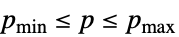
- 在 ParametricNDSolve[eqns,{u1,u2,…},…] 中,ui 可以是任意表达式. 通常,ui 间接通过微分方程的解依赖于参数,但是可能显式依赖于参数. 返回一个列表的 ParametricFunction 对象可以通过使用 ParametricNDSolve[eqns,{{u1,u2,…}},…] 或者使用 ParametricNDSolveValue[eqns,{u1,u2,…},…] 得到.
- 由此得出关于参数的 ParametricFunction 对象的导数会尽可能地组合使用符号和数值灵敏度方法进行计算.
- ParametricNDSolve 接受与 NDSolve 同样的选项和设置.
- 根据方程组的类型,NDSolve 和 ParametricNDSolve 通常通过多个不同的阶段求解微分方程组. 当 Method->{s1->m1,s2->m2,…} 时,阶段 si 由方法 mi 处理. 基于所要解决的问题,实际使用的阶段和顺序是由 NDSolve 决定的.
- 可能的解阶段与 NDSolve 是一样的,但还包括:
-
"ParametricCaching" 缓存计算的解 "ParametricSensitivity" 关于参数导数的计算
所有选项的列表
范例
打开所有单元 关闭所有单元基本范例 (3)
sol = ParametricNDSolve[{y'[t] == a y[t], y[0] == 1}, y, {t, 0, 10}, {a}]y1 = y[1] /. sol
y1[10] /. solPlot[Evaluate[Table[y[a][t] /. sol, {a, -1, 1, .1}]], {t, 0, 1}, PlotRange -> All]
sol = ParametricNDSolve[{y''[t] + a y[t] == 0, y[0] == 1, y'[0] == 0}, {y}, {t, 0, 10}, {a}]Plot[Evaluate[y[a][10] /. sol], {a, 0, 2}]FindRoot[y[a][10] /. sol, {a, 1}]sol = ParametricNDSolve[{y''[t] + a y[t] == 0, y[0] == b, y'[0] == 0}, y, {t, 0, 20}, {a, b}]Plot[Evaluate[(y[1, 1][t] + {0, .1, -.1}D[y[a, 1], a][t] /. a -> 1) /. sol], {t, 0, 20}, Filling -> {2 -> {3}}]Plot[Evaluate[(y[1, 1][t] + {0, .1, -.1}D[y[1, b], b][t] /. b -> 1) /. sol], {t, 0, 20}, Filling -> {2 -> {3}}]范围 (5)
参数相关性 (3)
ParametricNDSolve 返回 ParametricFunction 对象的一个替换:
sol = ParametricNDSolve[{y''[t] + y[t] == 3a Sin[y[t]], y[0] == y'[0] == 1}, y, {t, 0, 5}, {a}]
if0 = y[0] /. sol
Plot[if0[t], {t, 0, 5}]


Plot[Evaluate@Table[y[a][t] /. sol, {a, -.5, .5, .05}], {t, 0, 5}, PlotRange -> All]sol = ParametricNDSolve[{y''[t] + 2y[t] == Sin[.4t] + Cos[y[t]], y[0] == a, y'[0] == b}, y, {t, 0, 10}, {a, b}]


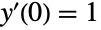
Plot[Evaluate@Table[y[a, 1][t] /. sol, {a, -2, 2, .5}], {t, 0, 10}, PlotRange -> All]


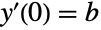
Plot[Evaluate@Table[y[1, b][t] /. sol, {b, -2, 2, .5}], {t, 0, 10}, PlotRange -> All]sol = ParametricNDSolve[{u''[x] == a u[x], DirichletCondition[u[x] == 1, x == 0], DirichletCondition[u[x] == b, x == 1]}, u, {x}∈Line[{{0}, {1}}], {a, b}]


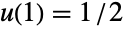
Plot[Evaluate@Table[u[a, 1 / 2][t] /. sol, {a, -2, 2, .5}], {t, 0, 10}, PlotRange -> All]参数灵敏度 (2)

sol = ParametricNDSolve[{y''[t] + y[t] == 0, y[0] == a, y'[0] == 0}, y, {t, 0, 10}, {a}];

y2 = y[2] /. sol;
Show[Plot[Evaluate@Table[y[a][t] /. sol, {a, 1, 3, .2}], {t, 0, 10}, PlotStyle -> Thin], Plot[y2[t], {t, 0, 10}]]


dy2 = y'[2] /. sol;
Plot[dy2[t], {t, 0, 10}]


Plot[Evaluate[y2[t] + {-1, 0, 1}dy2[t]], {t, 0, 10}, PlotStyle -> {Gray, {Blue}, Gray}, Filling -> {1 -> {3}}]sol = ParametricNDSolve[{y''[t] + 2y[t] == Sin[t] + Cos[y[t]], y[0] == a, y'[0] == b}, y, {t, 0, 10}, {a, b}];ifun = y[1, 1] /. sol


ifuna = D[y[a, 1], a] /. a -> 1 /. solPlot[Evaluate[ifun[t] + {-.5, 0, .5}ifuna[t]], {t, 0, 10}, PlotStyle -> {Gray, {Blue}, Gray}, Filling -> {1 -> {3}}]

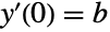
ifunb = D[y[1, b], b] /. b -> 1 /. sol;Plot[Evaluate[ifun[t] + {-.5, 0, .5}ifunb[t]], {t, 0, 10}, PlotStyle -> {Gray, {Blue}, Gray}, Filling -> {1 -> {3}}]推广和延伸 (1)
针对不同的 WorkingPrecision 值求解 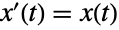 ,
,  并绘制误差:
sol = ParametricNDSolve[{x'[t] == x[t], x[0] == 1}, x[1], {t, 0, 1}, {wp}, Method -> "Extrapolation", WorkingPrecision -> wp ]ListLogPlot[Table[{wp, Abs[x[1][wp] - E] /. sol}, {wp, 16, 60}]]选项 (2)
Method (2)
ParametricCaching (1)
sol = ParametricNDSolve[{x''[t] + a x[t] == 0, x[0] == b, x'[0] == 0}, x, {t, 0, 1000}, {a, b}, MaxSteps -> ∞, Method -> {"ParametricCaching" -> None}];Do[Print[Module[{m = MemoryInUse[]},
AbsoluteTiming[{ByteCount[x[2, 2] /. sol], MemoryInUse[] - m}]]], {3}]


sol = ParametricNDSolve[{x''[t] + a x[t] == 0, x[0] == b, x'[0] == 0}, x, {t, 0, 1000}, {a, b}, MaxSteps -> ∞];Do[Print[Module[{m = MemoryInUse[]},
AbsoluteTiming[{ByteCount[x[2, 2] /. sol], MemoryInUse[] - m}]]], {3}]


ParametricSensitivity (1)
sol = ParametricNDSolve[{x'[t] == a x[t], x[0] == b}, x, {t, 0, 1}, {a, b}, Method -> {"ParametricSensitivity" -> None}];Plot3D[Evaluate[x[a, b][1] /. sol], {a, 1, 2}, {b, 0, 1}]dfun = Derivative[1, 0][x /. sol];
dfun[1, 1]
应用 (11)
参数扫描 (5)


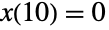
sol = ParametricNDSolve[{x''[t] - x'[t] + x[t] == 0, x[0] == 1, x'[0] == s}, x, {t, 0, 30}, {s}];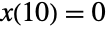
root = FindRoot[Evaluate[x[s][10] /. sol], {s, 6}]NDSolve[{x''[t] - x'[t] + x[t] == 0, x[0] == 1, x'[0] == s} /. root, x, {t, 0, 10}];Plot[x[t] /. %, {t, 0, 10}]Show[Plot[Evaluate@Table[Tooltip[x[s][t], s] /. sol, {s, 1, 1.8, 0.1}], {t, 0, 10}, PlotStyle -> Lighter[Gray, 0.5]],
Plot[Evaluate[x[s][t] /. sol /. root], {t, 0, 10}, PlotStyle -> Orange]]求边界值问题  ,
,  ,
, 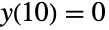 的多个解. 首先考虑
  的多个可能的值:
sol = ParametricNDSolve[{y''[t] + Sin[y[t]] == 0, y[0] == 0, y'[0] == s}, y, {t, 0, 10}, {s}];Plot[Evaluate@Table[Tooltip[y[s][t] /. sol, s], {s, 0.3, 1.9, 0.1}], {t, 0, 10}]
Plot[(y[s] /. sol)[10], {s, 0, 2.1}]val = Table[FindRoot[(y[s] /. sol)[10], {s, s0}], {s0, {0.9, 1.9, 2}}]Plot[Evaluate[y[s][t] /. sol /. val], {t, 0, 10}]求  的所有特征值
  和特征函数
和特征函数  ,其中
,其中  . 通过探索可能的参数值开始:
psol = y /. ParametricNDSolve[{y''[x] == -λ^2 y[x], y[0] == 0, y'[0] == λ}, y, {x, 0, 1}, {λ}];Plot[Evaluate@Table[Tooltip[psol[λ][x], λ], {λ, π / 2, 11π / 2, π / 2}], {x, 0, 1}]
pfun = y[1] /. ParametricNDSolve[{y''[x] == -λ^2 y[x], y[0] == 0, y'[0] == λ}, y[1], {x, 0, 1}, {λ}];Plot[pfun[λ], {λ, π / 2, 11π / 2}]sol = Table[FindRoot[pfun[λ] == 0, {λ, λ0}], {λ0, {3, 6, 9, 12, 16}}]//QuietPlot[Evaluate[psol[λ][x] /. sol], {x, 0, 1}]求  的值,满足
的值,满足  ,
,  的解在从
的解在从  到
到  范围内有最小弧长. 首先,绘制
  的值在从 0 到 1 范围内的解:
psol = ParametricNDSolve[{y''[t] + y[t] == 3a Sin[y[t]], y[0] == y'[0] == 1, α'[t] == Sqrt[1 + y[t] ^ 2], α[0] == 0}, {y, α}, {t, 0, 10}, {a}];Plot[Evaluate@Table[y[a][t] /. psol, {a, 0, 1, .1}], {t, 0, 10}]
Plot[Evaluate[α[a][10] /. psol], {a, 0, 1}, PlotPoints -> 100]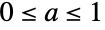

Show[Plot[Evaluate@Table[y[a][t] /. psol, {a, 0, 1, .1}], {t, 0, 10}, PlotRange -> All, PlotPoints -> 500, PlotStyle -> Lighter[Gray, 0.3]], Plot[Evaluate[y[0][t] /. psol], {t, 0, 10}, PlotStyle -> Thick]]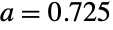
lmin = FindMinimum[α[a][10] /. psol, {a, 0.72}, AccuracyGoal -> 7]Show[{Plot[Evaluate@Table[y[a][t] /. psol, {a, .65, .8, .005}], {t, 0, 10}, PlotStyle -> Lighter[Gray, 0.5]], Plot[Evaluate[y[a][t] /. psol /. lmin[[2]]], {t, 0, 10}, PlotStyle -> Thick]}]求解径向形式的 Klein-Gordon 方程,势能形式为  :
:
sol = ParametricNDSolve[{Derivative[2][R][r] - ((1 - (UnitConvert[Quantity[1, "FineStructureConstant"]] E^-r Z + ϵ)^2) R[r]) == 0, R[0] == 0, R'[0] == 1}, R, {r, 0, 50}, {ϵ, Z}]


ContourPlot[(R[ϵ, Z][50] /. sol) == 0, {Z, 50, 800}, {ϵ, -1, 1}, FrameLabel -> Automatic, PlotPoints -> 100]参数灵敏度 (4)
pfun = y /. ParametricNDSolve[{y''[t] + y[t] == a Sin[2t ] + Cos[2y[t]], y[0] == 1, y'[0] == 0}, y, {t, 0, 10}, {a}];Show[Plot[Evaluate@Table[pfun[a][t], {a, -.6, .6, .1}], {t, 0, 5}, PlotStyle -> Lighter[Gray, 0.3], PlotRange -> All], Plot[pfun[0][t], {t, 0, 5}]]Plot[Evaluate[pfun[0][t] + {-.5, 0, .5}pfun'[0][t]], {t, 0, 5}, PlotStyle -> {Gray, {Blue}, Gray}, Filling -> {1 -> {3}}]pfun = θ /. ParametricNDSolve[{θ''[t] + (9.8 / 10)Sin[θ[t]] == -(a / 10)w ^ 2 Sin[w t]Sin[θ[t]], θ[0] == 3.14158, θ'[0] == 0.01}, θ, {t, 0, 5}, {w, a}];
if = pfun[50, 2];
ifa = D[pfun[w, a], a] /. {w -> 50, a -> 2};Plot[Evaluate[if[t] + {-.1, 0, .1}ifa[t]], {t, 0, 5}, PlotStyle -> {Gray, Blue, Gray}, Filling -> {1 -> {3}}]

pfun = u /. ParametricNDSolve[{D[u[t, x], t] == c^2 D[u[t, x], x, x], u[0, x] == Exp[-(a x) ^ 2], u[t, -10] == u[t, 10] == 0}, u, {t, 0, 5}, {x, -10, 10}, {a, c}];

ifun = pfun[1, 1];
ifda = D[pfun[a, 1], a] /. {a -> 1};
ifdc = D[pfun[1, c], c] /. {c -> 1};Panel@Grid[Join[{{"", "a", "c"}}, Table[{Row[{"t=", τ}], Plot[Evaluate[(ifun[τ, x] + .5{0, 1, -1}ifda[τ, x])], {x, -10, 10}, Filling -> {2 -> {3}}, PlotRange -> All], Plot[Evaluate[(ifun[τ, x] + .5{0, 1, -1}ifdc[τ, x])], {x, -10, 10}, Filling -> {2 -> {3}}, PlotRange -> All]}, {τ, {1, 3, 5}}]]]ColorSensitivityPlot3D[f_, fsense_, opts___] :=
Block[{fs = fsense}, Plot3D[f, {t, 0, 5}, {x, -10, 10}, Mesh -> None, ColorFunction -> Function[{t, x}, ColorData["LakeColors"][fs]], PlotPoints -> 60, ColorFunctionScaling -> False, opts]]{ColorSensitivityPlot3D[pfun[1, 1][t, x], 1.5Abs[ifda[t, x]], PlotLabel -> a, PlotRange -> All], ColorSensitivityPlot3D[pfun[1, 1][t, x], Abs[ifdc[t, x]], PlotLabel -> c, PlotRange -> All]}ndf = x[T] /. ParametricNDSolve[{Derivative[1][x][t] == -3 (x[t] - y[t]), Derivative[1][y][t] == -x[t] z[t] + a x[t] - y[t], Derivative[1][z][t] == x[t] y[t] - z[t], x[0] == z[0] == 0, y[0] == 1}, x[T], {t, 0, T}, {a, T}, MaxSteps -> ∞];Plot[Evaluate[RealExponent[D[ndf[a, 8], a]]], {a, 26, 27}, PlotRange -> All]参数拟合 (2)
{sol, samples} = NDSolve[{y''[t] == -9.8, y[0] == 1, y'[0] == 40, WhenEvent[Mod[t, .5] == 0, Sow[{t, y[t]}]]}, y, {t, 0, 10}]//Reap;
noisysamples = Map[({#[[1]], #[[2]] + RandomReal[{-10, 10}]})&, First@samples];ListPlot[noisysamples]pfun = y /. ParametricNDSolve[{y''[t] == -w y[t], y[0] == a, y'[0] == b}, y, {t, 0, 10}, {w, a, b}];fit = FindFit[noisysamples, pfun[w, a, b][t], {{w, .1}, {a, 1}, {b, 1}}, t]Plot[pfun[w, a, b][t] /. fit, {t, 0, 10}, Epilog -> {Point@noisysamples}]pfun = y /. ParametricNDSolve[{y''[t] == -g, y[0] == p, y'[0] == v}, y, {t, 0, 10}, {g, p, v}];fit = FindFit[noisysamples, pfun[g, p, v][t], {{g, 5}, {p, .5}, {v, .5}}, t]Plot[pfun[g, p, v][t] /. fit, {t, 0, 10}, Epilog -> {Point@noisysamples}]time = Quantity[{0, 25, 34, 42, 54, 63, 80, 89, 103, 115, 131, 145, 158, 175, 195, 213, 225, 250, 274, 298, 315, 335, 353, 387, 411, 440, 475, 492, 520, 530, 550, 560, 570, 585, 600, 610, 620, 630, 640, 647, 660, 670, 680, 690, 700, 710, 720, 730, 740, 750, 760, 770, 778, 790, 800, 810, 820, 830, 840, 850, 860, 870, 880, 890, 900, 910, 920, 930, 940, 950, 960, 970, 980, 990, 1000, 1010, 1020, 1030, 1040, 1050, 1060, 1070, 1080, 1090, 1100, 1110, 1120, 1130, 1140, 1150, 1160, 1170, 1180, 1190, 1200, 1210, 1220, 1230, 1240, 1250, 1260, 1270, 1280, 1300, 1340, 1356, 1380, 1418, 1725, 1740, 1825, 1890, 1955, 2022, 2077, 2160, 2244, 2320, 2408, 2473, 2613}, "Seconds"];
temp = Quantity[{210, 204, 200, 198, 196, 194, 192, 190, 188, 186, 184, 182, 180, 178, 176, 174, 172, 170, 168, 166, 164, 162, 160, 158, 156, 154, 152, 150, 150, 148, 148, 147, 146, 145, 144, 144, 144, 143, 143, 142, 142, 141, 141, 140, 140, 139.5, 139, 139, 138, 138, 137, 137, 136, 136, 136, 135, 135, 134, 134, 133, 133, 133, 132.5, 132, 132, 131, 131, 131, 130, 130, 129.5, 129, 129, 128.5, 128, 128, 128, 127.5, 127, 127, 126, 126, 126, 125.5, 125, 125, 124.5, 124, 124, 123.5, 123, 123, 122.5, 122, 122, 122, 121.5, 121, 121, 121, 120.5, 120.5, 120, 120, 119, 118, 117, 116, 111, 110.5, 109, 108, 107, 106, 105, 104, 103, 102, 101, 100, 99}, "DegreesFahrenheit"];BoltzmannConstant = Quantity[1.3806504`*^-23, "Joules" / "Kelvins"];tempK = UnitConvert[temp, "Kelvins"];
fitdata = QuantityMagnitude[Transpose[{time, tempK}]];
Subscript[tempK, 0] = QuantityMagnitude[First[tempK]];
Subscript[tempK, ∞] = QuantityMagnitude[UnitConvert[Quantity[79, "DegreesFahrenheit"], "Kelvins"]];c = QuantityMagnitude[(2260 18/6.02 10^23 BoltzmannConstant)];
tend = QuantityMagnitude[Last[time]];pfun = T /. ParametricNDSolve[{(Derivative[1][T][t] == -K1 (T[t] - Subscript[tempK, ∞]) - K2 (E^-c / T[t] - E^-c / Subscript[tempK, ∞])), T[0] == Subscript[tempK, 0]}, T, {t, 0, tend}, {K1, K2}];fit = FindFit[fitdata//N, pfun[K1, K2][t], {{K1, 0.0001}, {K2, 10000}}, t]Show[ListPlot[fitdata], Plot[Evaluate[pfun[K1, K2][t] /. fit], {t, 0, tend}, PlotStyle -> Red]]属性和关系 (1)
使用 SystemModelParametricSimulate 模拟更大的分层系统模型:
pf = SystemModelParametricSimulate[\!\(\*GraphicsBox[«8»]\), "Inertia2.w", 40, {"Resistor1.R", "SpringDamper1.d"}]sims = {pf[0.1, 0.25], pf[0.4, 0.3]};Plot[Evaluate@Comap[sims, t], {t, 0, 40}]文本
Wolfram Research (2012),ParametricNDSolve,Wolfram 语言函数,https://reference.wolfram.com/language/ref/ParametricNDSolve.html (更新于 2014 年).
CMS
Wolfram 语言. 2012. "ParametricNDSolve." Wolfram 语言与系统参考资料中心. Wolfram Research. 最新版本 2014. https://reference.wolfram.com/language/ref/ParametricNDSolve.html.
APA
Wolfram 语言. (2012). ParametricNDSolve. Wolfram 语言与系统参考资料中心. 追溯自 https://reference.wolfram.com/language/ref/ParametricNDSolve.html 年