


SystemModelCalibrate
SystemModelCalibrate[data,smodel,pars]
calibrates the parameters pars in the system model smodel according to data.
SystemModelCalibrate[data,{smodel,cons},pars]
calibrates the parameters pars subject to the constraints cons.
SystemModelCalibrate[…,spec]
calibrates following the specification spec.
SystemModelCalibrate[…,"prop"]
gives the value of the property "prop".
Details and Options
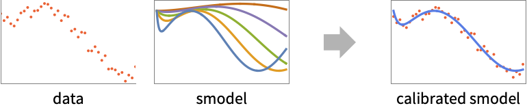
- SystemModelCalibrate is used to calibrate parameter values in a system model to match simulation results with real-world data.
- Given measured data
 from the real-world system, the goal is to calibrate parameters pars
  in the smodel to produce simulated data
  that is as close as possible to the measured data.
 - The calibrated parameters are
 , where
  are non-negative weights and ℓ is a loss function with typical form
  , which is approximated by the sampled data as
  .
. - Several quality measures of how well data and calibrated model agree can be computed as properties.
- The system model smodel can have the following forms:
-
SystemModel[…] general system model StateSpaceModel[…] state-space model TransferFunctionModel[…] transfer function model AffineStateSpaceModel[…] affine state-space model NonlinearStateSpaceModel[…] nonlinear state-space model DiscreteInputOutputModel[…] discrete input-output model - data is an association of the form <x1data1,…>, where xi is a variable in smodel and datai is its corresponding data.
- pars is a list of tunable parameters in smodel. It can have the following forms:
-
{θ1,…} calibration parameters starting from values in smodel {{θ1,  },…}
},…}calibration parameter θi starting from point 
- spec is an Association that allows the following keys:
-
"SimulationInterval" {tmin,tmax} simulate from time tmin to tmax "ParameterValues" {p1val1,…} parameter pi has value vali "InitialValues" {x1val1,…} variable xi has initial value vali "Inputs" {in1fun1,…} input ini has value funi[t] at time t "CalibratedModelName" name name for calibrated SystemModel "ExtendModel" False whether the calibrated SystemModel extends smodel "Weights" {w1,…} positive multi-objective sum weights wi for each calibration variable in data - The "CalibratedModelName" name can have the following forms:
-
Automatic automatically generate a model name (default) "name" name calibrated model "name" None set calibrated values in place in smodel - By default, SystemModelCalibrate[data,smodel,pars,spec] returns a model with parameters set to the calibrated values.
- SystemModelCalibrate[…,"CalibratedSystemModel"] returns a CalibratedSystemModel object csmodel that can be used to extract additional properties using the form csmodel["prop"].
- SystemModelCalibrate[…,"prop"] can be used to directly get the value of csmodel["prop"].
- Typical properties that can be retrieved with SystemModelCalibrate[…,"prop"] include:
-
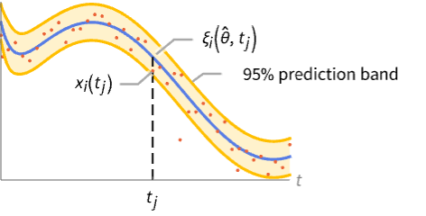
"CalibratedModel" new model with calibrated parameters "CalibratedParameters" parameter estimates "ParameterConfidence" parameter confidence information "MeanPredictionBandsPlot" mean predictions confidence bands plot with calibration data "SinglePredictionBandsPlot" plot of confidence bands based on single observations with calibration data - Properties related to data and the calibrated model include:
-
"CalibratedSimulationData" calibrated model simulation results "CalibrationData" calibration data in data "ValidationData" validation set data "CalibratedModelName" model name of new model with calibrated parameters "CalibrationDataResponse" response values in the calibration data "ValidationDataResponse" response values in the validation data "CalibratedDataResponse" calibrated model values for the calibration data "CalibratedValidationDataResponse" calibrated model values for the validation data - Types of residuals include:
-
"CalibrationDataResiduals" difference between actual and predicted responses "ValidationDataResiduals" difference between validation and predicted responses "StandardizedResiduals" residuals for calibration data divided by the standard error for each residual - Properties of predicted values include:
-
"CorrelationMatrix" asymptotic parameter correlation matrix "MeanPredictionBands" confidence bands for mean predictions "MeanPredictionConfidence" confidence information for the mean predictions of calibration data "SinglePredictionBands" confidence bands based on single observations "SinglePredictionConfidence" confidence information for the predicted response of single observations of calibration data - Properties that measure goodness of calibration include:
-
"MSE" mean squared error for each calibration variable, i.e. 
"RMSE" root mean squared error for each calibration variable, i.e. 
"RRMSE" relative root mean squared error for each calibration variable, i.e. 
- Properties that store calibration details include:
-
"CalibrationParameterConstraints" calibration parameter constraints cons "CalibrationVariables" calibration variables in data "InitialCalibrationParameters" calibration parameters pars and their calibration start values "InputModel" model smodel "InputModelName" model name of SystemModel smodel "SimulationInterval" simulation interval used in calibration - The following options can be given:
-
ConfidenceLevel 95/100 confidence level for parameters and predictions FitRegularization None regularization for pars Method Automatic what simulation and calibration methods to use NormFunction Norm the norm to minimize ProgressReporting $ProgressReporting control display of progress ValidationSet None validation data VarianceEstimatorFunction Automatic function for estimating the error variance - With ConfidenceLevel->p, probability-p confidence intervals are computed for parameter and prediction intervals.
- FitRegularization and NormFunction can be used to change the calibration target into
 , where
  is a regularization function, e.g.
 ![g(theta)=lambda TemplateBox[{theta, 2}, Norm2]^2](Files/SystemModelCalibrate.en/17.png "g(theta)=lambda TemplateBox[{theta, 2}, Norm2]^2") (Tikhonov) or
(Tikhonov) or ![g(theta)=lambda TemplateBox[{theta, 1}, Norm2]](Files/SystemModelCalibrate.en/18.png "g(theta)=lambda TemplateBox[{theta, 1}, Norm2]") (Lasso), and the loss function is given by
(Lasso), and the loss function is given by  , where
  is the norm function.
 - The following settings for ValidationSet can be given:
-
None use only the existing calibration data to measure quality (default) data validation set in the same form as calibration data data Scaled[frac] reserve a specified fraction of the calibration data for validation - With the setting VarianceEstimatorFunction->f, the common variance is estimated by f[res,w], where res is the list of residuals and w is the list of weights.
- Method settings take the form Method <"sub1"val1,…>.
- Method suboptions "subi" include:
-
"CalibrationMethod" Automatic calibration method "SimulationMethod" Automatic simulation method - "CalibrationMethod" settings are the same as the Method settings in FindMinimum.
- "SimulationMethod" settings are the same as the Method settings in SystemModelSimulate.
- Distributional assumptions are based on an unconstrained model calibrated by minimizing the default loss function.
Properties
Options
Examples
open all close allBasic Examples (2)
Use data of the angular velocity of a component to calibrate a model of a hybrid motor:
model = \!\(\*GraphicsBox[«8»]\);dataw = {...};Calibrate the values of the resistance and the damping:
cmodel = SystemModelCalibrate[<|"Inertia2.w" -> dataw|>, model, {"Resistor1.R", "SpringDamper1.d"}]Simulate with the calibrated parameters and compare with the data:
Show[SystemModelPlot[cmodel, {"Inertia2.w"}, 40], ListPlot[dataw, PlotStyle -> RGBColor[0.880722, 0.611041, 0.142051]], PlotRange -> All]Use data of an output of a NonlinearStateSpaceModel to calibrate the model:
nsys = NonlinearStateSpaceModel[{{u + a*Cos[Subscript[x, 2]] - Cos[Subscript[x, 1]*Subscript[x, 2]],
   -Cos[1 + Subscript[x, 2]] + Subscript[x, 1]}, {Subscript[x, 1]}},
{Subscript[x, 1], Subscript[x, 2]}, {u}, {Automatic}, Automatic, SamplingPeriod -> None];datay = {...};csmodel = SystemModelCalibrate[<|1 -> datay|>, nsys, {{a, 1}}, "CalibratedSystemModel"]Compute the single prediction bands and plot them together with the data and the calibrated simulation response:
csmodel["SinglePredictionBandsPlot"]//FirstScope (15)
Data (3)
Provide data for as many variables as you want to calibrate:
nsys = NonlinearStateSpaceModel[{{v, a + f - v -
    9*x}, {x}}, {x, v}, {f},
{Automatic}, Automatic, SamplingPeriod -> None];datax = {...};datav = {...};csmodel = SystemModelCalibrate[<|x -> datax, v -> datav|>, nsys, {a}, "CalibratedSystemModel"]Simulate with the calibrated parameter and compare with the data:
csmodel["SinglePredictionBandsPlot"]//DatasetUse data with units to calibrate a model of a rocket takeoff:
model = [image];datam = QuantityArray[IconizedObject[«data»], {"Seconds", "Kilograms"}];Calibrate the mass flow rate with data of the mass of the ship:
SystemModelCalibrate[<|"m" -> datam|>, {model, 0.39 < "k" < 0.46}, {"k"}, "CalibratedParameters"]Use the time-value pairs of a time series as data to calibrate a model:
nsys = NonlinearStateSpaceModel[
 {{a + Tanh[u - Subscript[x, 1]*
       Subscript[x, 2]], b +
    Tanh[a + u*Subscript[x, 2]]},
  {Subscript[x, 1]}}, {Subscript[x, 1], Subscript[x, 2]},
{u}, {Automatic}, Automatic, SamplingPeriod -> None];datay = TimeSeries[{...}];Calibrate the values of two parameters:
SystemModelCalibrate[<|1 -> datay|>, nsys, {a, b}]Models (4)
Use data generated with an input signal to calibrate a DiscreteInputOutputModel:
diom = DiscreteInputOutputModel[Association["SampledSeries" -> TemporalData[TimeSeries,
    {{{{a + u[0]}, {(u[0] + a*u[1])/2}, {(u[0] + a*u[1] + 2*a*u[2])/3}}}, {{0, 2, 1}}, 1,
     {"Discrete", 1}, {"Discrete", 1}, {1}, {MissingDataMethod -> None,
   ... ime", "LastValue", "OutputCount", "OutputVariables", "Path",
  "PathComponent", "PathComponents", "PathFunction", "PathLength", "SamplingPeriod", "StateCount",
"TemporalData", "TimePath", "Times", "TimeSeries", "TimeValues", "Type", "Values"}];datay = {...};input = Sin[Range[-5, 5]];Specify the input signal to calibrate a parameter value:
csmodel = SystemModelCalibrate[<|1 -> datay|>, diom, {a}, <|"Inputs" -> {1 -> input}|>, "CalibratedSystemModel"]Compute the single prediction bands and plot them together with the data and the calibrated simulation response:
csmodel["SinglePredictionBandsPlot"]//FirstUse data generated with an input signal to calibrate a TransferFunctionModel:
tfm = TransferFunctionModel[{{{2*(1 - a*s)}},
2*(1 + s/2 + s^2)}, s];datay = {...};input = UnitStep;Specify the input signal to calibrate a parameter value:
csmodel = SystemModelCalibrate[<|1 -> datay|>, tfm, {a}, <|"Inputs" -> {1 -> input}|>, "CalibratedSystemModel"]Compute the single prediction bands and plot them together with the data and the calibrated simulation response:
csmodel["SinglePredictionBandsPlot"]//FirstUse data generated with an input signal to calibrate a StateSpaceModel:
ssm = StateSpaceModel[{{{0, b}, {-a, -b}}, {{0}, {1}}, {{-1, 2}},
{{0}}}, SamplingPeriod -> None, SystemsModelLabels -> None];datay = {...};input = Tanh;Specify the input signal to calibrate parameter values:
csmodel = SystemModelCalibrate[<|1 -> datay|>, ssm, {{a, 1}, {b, 1}}, <|"Inputs" -> {1 -> input}|>, "CalibratedSystemModel"]Compute the single prediction bands and plot them together with the data and the calibrated simulation response:
csmodel["SinglePredictionBandsPlot"]//FirstUse data of the output of an AffineStateSpaceModel to calibrate the model:
assm = AffineStateSpaceModel[{{a*Cos[Subscript[x, 2]] -
    0.5*a*Cos[Subscript[x, 1]*Subscript[x, 2]],
   -Cos[1 + Subscript[x, 2]] + Subscript[x, 1]}, {{1}, {0}},
  {-Subscript[x, 1]}, {{0}}}, {Subscript[x, 1],
  Subscript[x, 2]}, {{u, 0}}, {Automatic}, Automatic,
SamplingPeriod -> None];datay = {...};csmodel = SystemModelCalibrate[<|1 -> datay|>, assm, {{a, 1}}, "CalibratedSystemModel"]Compute the single prediction bands and plot them together with the data and the calibrated simulation response:
csmodel["SinglePredictionBandsPlot"]//FirstParameters and Constraints (3)
Indicate initial guess values for the calibration parameters:
nsys = NonlinearStateSpaceModel[
 {{a + Tanh[u - Subscript[x, 1]*
       Subscript[x, 2]], b +
    Tanh[a + u*Subscript[x, 2]]},
  {Subscript[x, 1]}}, {Subscript[x, 1], Subscript[x, 2]},
{u}, {Automatic}, Automatic, SamplingPeriod -> None];datay = {...};Calibrate two parameter values:
SystemModelCalibrate[<|1 -> datay|>, nsys, {{a, 0.7}, {b, -0.5}}]Introduce constraints for the calibration parameters:
nsys = NonlinearStateSpaceModel[
 {{a + Tanh[u - Subscript[x, 1]*
       Subscript[x, 2]], b +
    Tanh[a + u*Subscript[x, 2]]},
  {Subscript[x, 1]}}, {Subscript[x, 1], Subscript[x, 2]},
{u}, {Automatic}, Automatic, SamplingPeriod -> None];datay = {...};Calibrate two parameter values:
csmodel = SystemModelCalibrate[<|1 -> datay|>, {nsys, 0.75 < a < 0.8, -0.6 < b < -0.55}, {{a, 0.77}, {b, -0.57}}, "CalibratedSystemModel"]Confidence intervals are computed assuming an unconstrained model:
csmodel["ParameterConfidence"]Introduce constraints for the calibration parameters when fitting several variables:
nsys = NonlinearStateSpaceModel[{{v, a + f - v -
    9*x}, {x}}, {x, v}, {f},
{Automatic}, Automatic, SamplingPeriod -> None];datax = {...};datav = {...};SystemModelCalibrate[<|x -> datax, v -> datav|>, {nsys, 0.5 < a < 1.5}, {{a, 1}}]Specification (4)
Specify a model name for the calibrated model:
model = [image];datay = {...};Calibrate the value of a parameter, specifying the calibrated model name:
SystemModelCalibrate[<|"y" -> datay|>, {model, 3 < "a" < 5}, {{"a", 4}}, <|"CalibratedModelName" -> "MyCalibratedModel"|>]Create a calibrated model that extends the input model:
cmodel = SystemModelCalibrate[<|"y" -> datay|>, {model, 3 < "a" < 5}, {{"a", 4}}, <|"CalibratedModelName" -> "ExtendsInputModel", "ExtendModel" -> True|>]cmodel["ExtendsModels"]Use data generated with an input signal to calibrate a model:
ssm = StateSpaceModel[{{{0, b}, {-a, -b}}, {{0}, {1}}, {{-1, 2}},
{{0}}}, SamplingPeriod -> None, SystemsModelLabels -> None];datay = {...};input = Tanh;Specify the input signal to calibrate parameter values:
SystemModelCalibrate[<|1 -> datay|>, ssm, {{a, 1}, {b, 1}}, <|"Inputs" -> {1 -> input}|>]Specify a fixed value for a parameter to calibrate another:
SystemModelCalibrate[<|1 -> datay|>, ssm, {{a, 1}}, <|"Inputs" -> {1 -> input}, "ParameterValues" -> {b -> 1.54}|>]Specify initial values and a simulation interval to calibrate a model:
assm = AffineStateSpaceModel[{{a*Cos[Subscript[x, 2]] -
    0.5*a*Cos[Subscript[x, 1]*Subscript[x, 2]],
   -Cos[1 + Subscript[x, 2]] + Subscript[x, 1]}, {{1}, {0}},
  {-Subscript[x, 1]}, {{0}}}, {Subscript[x, 1],
  Subscript[x, 2]}, {{u, 0}}, {Automatic}, Automatic,
SamplingPeriod -> None];datay = {...};SystemModelCalibrate[<|1 -> datay|>, assm, {{a, 1}}, <|"InitialValues" -> {Subscript[x, 1] -> 0.01}, "SimulationInterval" -> {0, 5}|>]Provide weights for the calibration of several variables:
nsys = NonlinearStateSpaceModel[{{v, a + f - v -
    9*x}, {x}}, {x, v}, {f},
{Automatic}, Automatic, SamplingPeriod -> None];datax = {...};datav = {...};weights = {1, 2};csmodel = SystemModelCalibrate[<|x -> datax, v -> datav|>, nsys, {a}, <|"Weights" -> weights|>, "CalibratedSystemModel"]Compute the single prediction bands and plot them together with the data and the calibrated simulation response:
csmodel["SinglePredictionBandsPlot"]//DatasetProperties (1)
Find the list of available properties:
nsys = NonlinearStateSpaceModel[{{u + a*Cos[Subscript[x, 2]] -
    Cos[Subscript[x, 1]*Subscript[x, 2]],
   -Cos[1 + Subscript[x, 2]] + Subscript[x, 1]},
  {Subscript[x, 1]}}, {Subscript[x, 1], Subscript[x, 2]},
{u}, {Automatic}, Automatic, SamplingPeriod -> None];datay = {...};SystemModelCalibrate[<|1 -> datay|>, nsys, {{a, 1}}, "Properties"]//ShallowThese can be extracted more conveniently from the CalibratedSystemModel:
csmodel = SystemModelCalibrate[<|1 -> datay|>, nsys, {{a, 1}}, "CalibratedSystemModel"]csmodel["Properties"]Extract the single prediction bands plot:
csmodel["SinglePredictionBandsPlot"]//FirstExtract the single prediction bands plot with a custom confidence level:
csmodel["SinglePredictionBandsPlot", ConfidenceLevel -> 0.5]//FirstExtract the single prediction bands plot with a custom variance estimator function:
csmodel["SinglePredictionBandsPlot", VarianceEstimatorFunction -> (Mean[Abs[#]]&)]//FirstExtract the calibrated model and the calibrated parameters:
csmodel[{"CalibratedModel", "CalibratedParameters"}]Extract the single prediction bands:
csmodel["SinglePredictionBands"]//ShortExtract the single prediction bands evaluated at time t:
csmodel["SinglePredictionBands", t]//ShortExtract the root mean squared error for each calibration variable:
csmodel["MSE"]Extract the root mean squared error for each calibration variable providing a validation set:
csmodel["MSE", ValidationSet -> <|1 -> {{2.6, 1.8}, {2.7, 1.56}, {2.8, 1.4}, {2.9, 1.2}, {3., 1.2}, {3.1, 1.0}, {3.2, 1.0}, {3.3, 0.8}}|>]Extract parameter confidence information, including estimates, standard errors, confidence intervals,
csmodel["ParameterConfidence"]Options (8)
ConfidenceLevel (1)
Use data of the states of a model to calibrate a parameter:
nsys = NonlinearStateSpaceModel[{{v, a + f - v -
    9*x}, {x}}, {x, v}, {f},
{Automatic}, Automatic, SamplingPeriod -> None];datax = {...};datav = {...};Use the default confidence level:
SystemModelCalibrate[<|x -> datax, v -> datav|>, nsys, {a}, "SinglePredictionBandsPlot"]Specify a custom confidence level of 0.5:
SystemModelCalibrate[<|x -> datax, v -> datav|>, nsys, {a}, "SinglePredictionBandsPlot", ConfidenceLevel -> 0.5]FitRegularization (1)
Use data of an output to calibrate a model:
nsys = NonlinearStateSpaceModel[
 {{a + Tanh[u - Subscript[x, 1]*
       Subscript[x, 2]], b +
    Tanh[a + u*Subscript[x, 2]]},
  {Subscript[x, 1]}}, {Subscript[x, 1], Subscript[x, 2]},
{u}, {Automatic}, Automatic, SamplingPeriod -> None];datay = {...};Use a loss function with no regularization to calibrate parameters:
SystemModelCalibrate[<|1 -> datay|>, nsys, {a, b}, "CalibratedParameters"]Use a Lasso regularization to calibrate parameters:
SystemModelCalibrate[<|1 -> datay|>, nsys, {a, b}, "CalibratedParameters", FitRegularization -> {"LASSO", 2}]Use a Tikhonov regularization to calibrate parameters:
SystemModelCalibrate[<|1 -> datay|>, nsys, {a, b}, "CalibratedParameters", FitRegularization -> {"Tikhonov", 2}]Method (2)
Use data of the mass of a ship to calibrate a model of a rocket takeoff:
model = [image];datam = IconizedObject[«data»];Use the default simulation method to calibrate the value of the mass flow rate:
SystemModelCalibrate[<|"m" -> datam|>, {model, 0.39 < "k" < 0.46}, {"k"}, "SinglePredictionBandsPlot"]//FirstCalibrate, specifying a number of interpolation points for simulation:
SystemModelCalibrate[<|"m" -> datam|>, {model, 0.39 < "k" < 0.46}, {"k"}, "SinglePredictionBandsPlot", Method -> <|"SimulationMethod" -> {"InterpolationPoints" -> 6}|>]//FirstUse data of an output to calibrate a model:
nsys = NonlinearStateSpaceModel[
 {{a + Tanh[u - Subscript[x, 1]*
       Subscript[x, 2]], b +
    Tanh[a + u*Subscript[x, 2]]},
  {Subscript[x, 1]}}, {Subscript[x, 1], Subscript[x, 2]},
{u}, {Automatic}, Automatic, SamplingPeriod -> None];datay = {...};Use the default fitting method to calibrate parameters:
csmodel = SystemModelCalibrate[<|1 -> datay|>, nsys, {a, b}, "CalibratedSystemModel"];csmodel["CalibratedParameters"]csmodel["SinglePredictionBandsPlot"]//FirstUse the conjugate gradient method to calibrate parameters:
csmodelg = SystemModelCalibrate[<|1 -> datay|>, nsys, {a, b}, "CalibratedSystemModel", Method -> <|"CalibrationMethod" -> "ConjugateGradient"|>];csmodelg["CalibratedParameters"]csmodelg["SinglePredictionBandsPlot"]//FirstNormFunction (1)
Use data of an output to calibrate a model:
nsys = NonlinearStateSpaceModel[
 {{a + Tanh[u - Subscript[x, 1]*
       Subscript[x, 2]], b +
    Tanh[a + u*Subscript[x, 2]]},
  {Subscript[x, 1]}}, {Subscript[x, 1], Subscript[x, 2]},
{u}, {Automatic}, Automatic, SamplingPeriod -> None];datay = {...};Use the default norm in the loss function to calibrate parameters:
SystemModelCalibrate[<|1 -> datay|>, nsys, {a, b}, "CalibratedParameters"]Use the ![]() -norm in the loss function to calibrate parameters:
-norm in the loss function to calibrate parameters:
SystemModelCalibrate[<|1 -> datay|>, nsys, {a, b}, "CalibratedParameters", NormFunction -> (Norm[#, Infinity]&)]Use the 1-norm in the loss function to calibrate parameters
SystemModelCalibrate[<|1 -> datay|>, nsys, {a, b}, "CalibratedParameters", NormFunction -> (Norm[#, 1]&)]ProgressReporting (1)
Use data of the mass of a ship to calibrate a model of a rocket takeoff:
model = [image];datam = IconizedObject[«data»];Calibrate the value of the mass flow rate with the default progress reporting:
SystemModelCalibrate[<|"m" -> datam|>, {model, 0.39 < "k" < 0.46}, {"k"}, "CalibratedParameters"]Calibrate without progress reporting:
SystemModelCalibrate[<|"m" -> datam|>, {model, 0.39 < "k" < 0.46}, {"k"}, "CalibratedParameters", ProgressReporting -> False]ValidationSet (1)
Use data of an output to calibrate a model:
nsys = NonlinearStateSpaceModel[
 {{a + Tanh[u - Subscript[x, 1]*
       Subscript[x, 2]], b +
    Tanh[a + u*Subscript[x, 2]]},
  {Subscript[x, 1]}}, {Subscript[x, 1], Subscript[x, 2]},
{u}, {Automatic}, Automatic, SamplingPeriod -> None];datay = {...};Calibrate parameters using no validation data:
SystemModelCalibrate[<|1 -> datay|>, nsys, {a, b}, "RMSE"]Calibrate parameters by reserving a fraction of the calibration data for validation:
SystemModelCalibrate[<|1 -> datay|>, nsys, {a, b}, "RMSE", ValidationSet -> Scaled[0.1]]Use a particular random seed in the selection of validation data to ensure predictable results:
BlockRandom[SystemModelCalibrate[<|1 -> datay|>, nsys, {a, b}, "RMSE", ValidationSet -> Scaled[0.1]], RandomSeeding -> 1234]Use a custom validation set to calibrate parameters:
SystemModelCalibrate[<|1 -> datay|>, nsys, {a, b}, "RMSE", ValidationSet -> <|1 -> {{0.75, 0.9}, {1., 0.7}, {1.25, 1.1}, {1.5, 1.2}, {1.75, 1.15}}|>]VarianceEstimatorFunction (1)
Use data of the states of a model to calibrate a parameter:
nsys = NonlinearStateSpaceModel[{{v, a + f - v -
    9*x}, {x}}, {x, v}, {f},
{Automatic}, Automatic, SamplingPeriod -> None];datax = {...};datav = {...};Use the default estimate of error variance:
SystemModelCalibrate[<|x -> datax, v -> datav|>, nsys, {a}, "SinglePredictionBandsPlot"]Estimate the variance by the mean absolute error:
SystemModelCalibrate[<|x -> datax, v -> datav|>, nsys, {a}, "SinglePredictionBandsPlot", VarianceEstimatorFunction -> (Mean[Abs[#]]&)]Applications (5)
Industrial Manufacturing (1)
Use temperature data to estimate the heat transfer coefficient in a model of a continuous stirred-tank reactor:
model = [image];Use the measured temperature of the tank and the cooling medium:
dataTr = QuantityArray[IconizedObject[«dataTr»], {"Hours", "Kelvins"}];
dataTj = QuantityArray[IconizedObject[«dataTj»], {"Hours", "Kelvins"}];
Set the cooling medium flow rate used in the measurement as input:
mediumFlowRate = <|"Inputs" -> {"FJ" -> Function[0.02]}|>;Fit the heat transfer coefficient:
csmodel = Quiet[SystemModelCalibrate[<|"TR" -> dataTr, "TJ" -> dataTj|>, model, {"U"}, mediumFlowRate, "CalibratedSystemModel", Method -> <|"CalibrationMethod" -> "PrincipalAxis"|>], {FindMinimum::fmmp}]Compute the single prediction bands and plot them together with the data and the calibrated simulation response:
csmodel["SinglePredictionBandsPlot"]//DatasetPlot the residuals against time for the tank temperature:
ListPlot[Transpose[{dataTr[[All, 1]], csmodel["CalibrationDataResiduals"]["TR"]}], Sequence[Frame -> True, Filling -> Axis, FrameLabel -> {"h", "residual TR"}, PlotLabel -> "Residual vs Time"]]Model Simplification (1)
Recreate the behavior of a speaker by calibrating a simpler circuit using simulation results as input data:
speaker = [image];rl = [image];Compare the behavior of both models before calibration:
sims = SystemModelSimulate[speaker];simrl = SystemModelSimulate[rl];SystemModelPlot[{sims, simrl}, {"vs.v"}]Retrieve simulation results as data and use them for calibration:
datav = sims["RawData", "vs.v"];csmodel = SystemModelCalibrate[<|"vs.v" -> datav|>, {rl, 0.001 < l < 0.5}, {l}, "CalibratedSystemModel"]Compare the calibrated model with the speaker:
SystemModelPlot[{sims, csmodel["CalibratedSimulationData"]}, {"vs.v"}]Conveyor Belt Friction (1)
Calibrate the viscous contribution to friction in a model of a body held by a spring on top of an accelerating conveyor belt:
beltv[t_] := vb + ab t;The total kinetic friction can be modeled as a combination of viscous, Coulomb and Stribeck components:
viscous[v_] := -d (v - beltv[t]);coulomb[v_] := -c Sign[v - beltv[t]];stribeck[v_] := -s Sign[v] Exp[-σ Abs[v]];friction[v_] := viscous[v] + coulomb[v] + stribeck[v];The equations of motion must include the event-generating effect of the static friction, which holds the body static with respect to the belt until an upper bound is breached by external forces:
spring[x_] := -k (x - l);eqs = {m v'[t] == If[stuck[t] == 1, m beltv'[t], spring[x[t]] + friction[v[t]]],
x'[t] == v[t], WhenEvent[v[t] == beltv[t], stuck[t] -> Boole[spring[x[t]]^2 < μ^2]], WhenEvent[spring[x[t]]^2 > μ^2, stuck[t] -> 0]};Set initial values for the position and velocity of the body and the discrete variable tracking the impact of static friction:
initeqs = {x[0] == 1, v[0] == 0, stuck[0] == 0};Set parameter values and create the system model:
parVals = {m -> 1, l -> 1, d -> 5, c -> 5, s -> 1, μ -> 100, k -> 1000, σ -> 2, vb -> 1 / 10, ab -> 1 / 100};model = CreateSystemModel["ConveyorBeltFriction", Join[eqs, initeqs], t, <|"DiscreteVariables" -> {stuck}, "ParameterValues" -> parVals|>]Calibrate the contribution of the viscous term with data for the position of the body:
datax = {...};csmodel = SystemModelCalibrate[<|x -> datax|>, {model, 1 < d < 20}, {d}, "CalibratedSystemModel"]Find the 95% confidence interval for the viscous friction factor:
csmodel["ParameterConfidence"]Compute the single prediction bands and plot them together with the data and the calibrated simulation response:
csmodel["SinglePredictionBandsPlot"]//FirstCompute the extremes of the position and velocity for the calibrated simulation data:
SystemModelMeasurements[csmodel["CalibratedSimulationData"], {"MinValue", "MaxValue"}]Reverse Engineering of Controller (1)
Deduce the controller parameters in a controlled system for which you have step response data:
plant = TransferFunctionModel[{{{6}}, (1 + 2*s)*(1 + 4*s)*
(1. + 6*s)}, s];csys = PIDTune[plant, "PID", "ReferenceOutput"];sim = SystemModelSimulate[csys, 50, <|"Inputs" -> {1 -> UnitStep}|>];data = sim["RawData", Subscript[, 1]];Connect the plant model to a controller with symbolic parameters:
pid = TransferFunctionModel[{{{s^2*Subscript[k, d] +
     Subscript[k, i] + s*Subscript[k,
p]}}, s}, s];csysWithPars = SystemsModelFeedbackConnect[SystemsModelSeriesConnect[pid, plant]];Calibrate the parameters in the model with the step response data of the controlled system:
csmodel = SystemModelCalibrate[<|1 -> data|>, {csysWithPars, 0.01 < Subscript[k, p] < 10, 0.01 < Subscript[k, i] < 10, 0.01 < Subscript[k, d] < 10}, {{Subscript[k, p], 0.5}, {Subscript[k, i], 1}, {Subscript[k, d], 1}}, <|"Inputs" -> {1 -> UnitStep}|>, "CalibratedSystemModel"]Compare the simulation results of the calibrated model with the reverse-engineered model:
SystemModelPlot[{sim, csmodel["CalibratedSimulationData"]}, {Subscript[, 1]}, PlotStyle -> {Automatic, Directive[RGBColor[0.922526, 0.385626, 0.209179], Dashed]}, PlotRange -> All]Reduced Three-Body Problem (1)
Estimate the mass of a planet that orbits a star from the trajectory of one of its moons in a reduced three-body planetary system:
starPlanetSystemEqs = {μ12 r[t]^2θ'[t] == Sqrt[a (1 - e^2) 𝒢 m1 m2 μ12], r[t] == (a(1 - e^2)/1 + e Cos[θ[t] - θr]), {x1[t], y1[t]} == -(m2/m1 + m2){xr[t], yr[t]}, {x2[t], y2[t]} == (m1/m1 + m2){xr[t], yr[t]}, {xr[t], yr[t]} == r[t]{Cos[θ[t]], Sin[θ[t]]}};The dynamics of the moon are dictated by Newtonian gravity:
moonEqs = {m3 vx3'[t] == -𝒢 m1 m3(x3[t] - x1[t]/((x3[t] - x1[t])^2 + (y3[t] - y1[t])^2)^3 / 2) - 𝒢 m2 m3(x3[t] - x2[t]/((x3[t] - x2[t])^2 + (y3[t] - y2[t])^2)^3 / 2), m3 vy3'[t] == -𝒢 m1 m3(y3[t] - y1[t]/((x3[t] - x1[t])^2 + (y3[t] - y1[t])^2)^3 / 2) - 𝒢 m2 m3(y3[t] - y2[t]/((x3[t] - x2[t])^2 + (y3[t] - y2[t])^2)^3 / 2), {vx3[t], vy3[t]} == {x3'[t], y3'[t]}};Set parameter values for the system and initial values for the trajectory of the moon:
parVals = {𝒢 -> 1, m1 -> 1, m2 -> 0.0059, m3 -> 0.00001, a -> 1, e -> 0.0549, θr -> 0, μ12 -> (m1 m2/m1 + m2)};initVals = {x3 -> 0.9, vy3 -> 0.6};Create a model from the equations, parameters and initial values:
model = CreateSystemModel["ReducedTBP", Join[starPlanetSystemEqs, moonEqs], t, <|"ParameterValues" -> parVals, "InitialValues" -> initVals|>]Simulate the model before calibration and plot the trajectories of the three bodies:
sim = SystemModelSimulate[model, 4];ParametricPlot[Evaluate[{sim[{x1, y1}, t], sim[{x2, y2}, t], sim[{x3, y3}, t]}], {t, 0, 4}, ...]Calibrate a model with data for the trajectory of the moon:
datax3 = {...};datay3 = {...};csmodel = SystemModelCalibrate[<|x3 -> datax3, y3 -> datay3|>, {model, 0.001 < m2 < 0.007}, m2, "CalibratedSystemModel", Method -> <|"CalibrationMethod" -> "NMinimize"|>]Retrieve the simulation data and plot the trajectories for the calibrated model:
simcal = csmodel["CalibratedSimulationData"];cPlot = ParametricPlot[Evaluate[{simcal[{x1, y1}, t], simcal[{x2, y2}, t], simcal[{x3, y3}, t]}], {t, 0, 4}, ...]Compare the data with the calibrated trajectory:
Show[cPlot, ListPlot[Transpose[{datax3[[All, 2]], datay3[[All, 2]]}], PlotStyle -> RGBColor[0.922526, 0.385626, 0.209179], PlotLegends -> {"data"}]]Related Links
Text
Wolfram Research (2023), SystemModelCalibrate, Wolfram Language function, https://reference.wolfram.com/language/ref/SystemModelCalibrate.html.
CMS
Wolfram Language. 2023. "SystemModelCalibrate." Wolfram Language & System Documentation Center. Wolfram Research. https://reference.wolfram.com/language/ref/SystemModelCalibrate.html.
APA
Wolfram Language. (2023). SystemModelCalibrate. Wolfram Language & System Documentation Center. Retrieved from https://reference.wolfram.com/language/ref/SystemModelCalibrate.html