|
8.1.1 Identification Using Markov Parameters
The Hankel matrices of Markov parameters are defined as
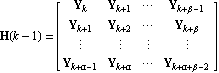
where  , ,  , ,  , ... are Markov parameters given by , ... are Markov parameters given by

The Markov parameters  , ,  , ,  can be constructed from the given impulse responses without explicit knowledge of the system matrices can be constructed from the given impulse responses without explicit knowledge of the system matrices  , ,  , ,  , and , and  . If the order of the system to be identified is . If the order of the system to be identified is  , then the choices of , then the choices of  and and  ensure that the matrix ensure that the matrix  is of rank is of rank  . .
If  is the singular value decomposition of the Hankel matrix is the singular value decomposition of the Hankel matrix  , then the matrices of the minimal state-space realization could be identified as , then the matrices of the minimal state-space realization could be identified as
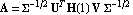 , ,  , , 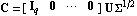 , , 
where  is the number of inputs and is the number of inputs and  is the number of outputs (see Juang (1994) for details). is the number of outputs (see Juang (1994) for details).


Time-domain system identification using the impulse responses.
For the single-input, single-output (SISO) systems, the response data is simply given as a list of the values  measured as the output to the unit impulse input sequence measured as the output to the unit impulse input sequence  . .
For the multi-input, multi-output (MIMO) systems, the response data is collected as follows. The first element of the list is taken as the output of the system when the unit impulse sequence to the first input and the zero sequence to all other inputs are applied. Then, after the system comes to rest, the second element of the list is taken as the output of the system, obtained by applying the unit impulse sequence to the second input and the zero sequence to all other inputs, and so on. Thus, the list of impulse response matrices, representing the responses for the unit impulse to the 1st, 2nd, ... inputs, is constructed in the same way as the one returned by the function OutputResponse, described in Section 4.2 of Control System Professional.


The format of impulse responses.
Using the option Sampled in the function ImpulseResponseIdentify passes the sampling period to the resulting state-space system. Otherwise, the sampling period is determined by the global value $SamplingPeriod similar to the convention used for the function ToDiscreteTime (Section 3.5 in Control System Professional).
Two options affect the number of states  of the system to be identified that could be used together or separately. The option value MaxOrder of the system to be identified that could be used together or separately. The option value MaxOrder  specifies the a priori known upper bound on the number of states specifies the a priori known upper bound on the number of states  . This option is suitable, for example, if a mechanical system with a known number of components is to be identified. Such an upper bound, when known, simplifies the computations. If no reasonable upper bound on the states is known, then the option value MaxOrderInfinity is used. The option Tolerance specifies the tolerance to be used to determine the number of Hankel singular values of the . This option is suitable, for example, if a mechanical system with a known number of components is to be identified. Such an upper bound, when known, simplifies the computations. If no reasonable upper bound on the states is known, then the option value MaxOrderInfinity is used. The option Tolerance specifies the tolerance to be used to determine the number of Hankel singular values of the  strong states that need to be kept in the identified model (see Section 7.1). Tolerance t specifies that weak modes with the Hankel singular values smaller than t times the maximum Hankel singular value are to be removed. With the default setting ToleranceAutomatic, strong states that need to be kept in the identified model (see Section 7.1). Tolerance t specifies that weak modes with the Hankel singular values smaller than t times the maximum Hankel singular value are to be removed. With the default setting ToleranceAutomatic,  is taken to be is taken to be  , where , where  is the precision of the input data. is the precision of the input data.
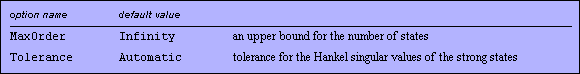
Options to determine the number of states in the identified system.
Make sure the application is loaded.
In[1]:=
Load the collection of test examples.
In[2]:=
This is a discrete-time state-space model of a steam power system.
In[3]:=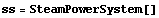
Out[3]=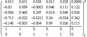
The specified number of measurements is  . .
In[4]:=
The built-in function Short displays only a skeleton of the simulated impulse responses.
In[5]:=
Out[5]//Short=
This identifies a minimal state-space realization using the derived impulse responses.
In[6]:=
Out[6]=
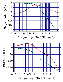
This Bode plot depicts the original and identified models by solid and dashed lines, respectively.
In[7]:=
In[8]:=
|