|
Cash Flows
Cash flows are more general finance objects than bonds. An individual cash flow is represented by an ordered pair {time, amount}. The time of a flow can be expressed either as a date or as a time interval from a given initial date.


CashFlows object.
First we load the Finance package.
In[1]:=<< Finance`
Here is a cash flows object.
In[2]:=cflows1 = CashFlows[{
{{2, 12, 1994}, 100 USDollar},
{{3, 15, 1994}, 300 USDollar},
{{3, 15, 1995}, 300 USDollar},
{{7, 1, 1995}, 150 USDollar},
{{10, 30, 1995}, 200 USDollar}}
];


Basic cash flows functions.
If we want to use the flat interest rates model, we take rates to be a single number—the yield to maturity. Otherwise for a term structure of interest rates the third argument is an interest rates object. In this section we assume that time intervals are expressed in years. This also applies to the other functions in the package that have interest rates as an argument.
We define an interest rates object rates1.
In[3]:=rates1 = DiscountFactors[{{1, 0.91805},
{2, 0.84566},
{3, 0.77461},
{5, 0.65892},
{7, 0.55676},
{10, 0.41714},
{30, 0.06779}},
InitialDate -> {1, 1, 1992}];
We assume the settlement day is September 15, 1993.
In[4]:=settlement = {9, 15, 1993}
Out[4]=
Here is the value of cflows1 on August 15, 1993, assuming that the yield to maturity is 12%.
In[5]:=val1 = Value[cflows1, settlement, .12]
Out[5]=
In this case, Mathematica recognizes that rates1 is an interest rates object and calculates the present value for the given structure of interest rates.
In[6]:=val2 = Value[cflows1, settlement, rates1]
Out[6]=
We can always create a cash flows finance object that is equivalent to a given bond. We redefine bond10.
In[7]:=bond10 = Bond[{.10, {9, 15, 2003}, 1000 USDollar, 2}];
We compute the cash flows dates for this bond.
In[8]:=flowDates = CashFlowsDates[bond10, {9, 30, 1993}]
Out[8]=
Next we create a list of amounts for the cash flows.
In[9]:=flowAmounts = Append[Table[50 USDollar,
{Length[flowDates]-1}], 1050 USDollar]
Out[9]=
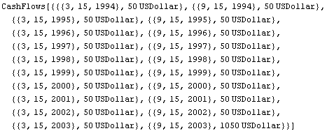
Finally we get a cash flows object that is equivalent to bond10.
In[10]:=cflows2 = CashFlows[Transpose[{flowDates, flowAmounts}]]
Out[10]=
The value of cflows2 should be identical to that of bond10.
In[11]:=val3 = Value[cflows2, settlement, .12]
Out[11]=
There is a discrepancy.
In[12]:=val4 = Value[bond10, settlement, .12]
Out[12]=
The first reason is the difference between the effective and nominal rates. In the value of cash flows, we are using annual rates although bond10 pays semiannually. Here is the correct annual rate.
In[13]:=effrate = NominalRate[12/100, 2, 1] // N
Out[13]=
We get slightly better agreement.
In[14]:=val5 = Value[cflows2, settlement, effrate]
Out[14]=
The second reason is that in the case of cash flows calculation, the time intervals are not necessarily equal since we use the actual calendar day count.
In[15]:=YearsBetween[{9, 15, 1994}, {3, 15, 1994}]
Out[15]=
The time periods are not exactly half-years, as we assume with bonds. Defining the time intervals to be  , 1, , 1,  , ... will make the results for bonds and their equivalent cash flows agree. , ... will make the results for bonds and their equivalent cash flows agree.
In[16]:=YearsBetween[{3, 15, 1995}, {9, 15, 1994}]
Out[16]=
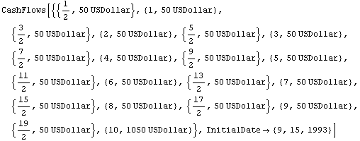
We define a new object that takes this into account. Here the dates in the cash flows object have been replaced by time intervals starting at a given initial date.
In[17]:=cflows3 = CashFlows[Append[Table[{i, 50 USDollar},
{i, 1/2, 9 + 1/2, 1/2}], {10, 1050 USDollar}],
InitialDate -> {9, 15, 1993}]
Out[17]=
Here is the value of cashflow3. It is equal to val4, as it should be.
In[18]:=val5 = Value[cflows3, settlement, effrate]
Out[18]=
This is the value of the cash flows object, equivalent to bond10 using the interest rates object rates1.
In[19]:=val6 = Value[cflows3, settlement, rates1]
Out[19]=


Additional cash flows function.
Now we compute the yield to maturity for cflows1, cflows2, and cflows3 using the prices val1, val3, and val5. We get the expected results.
In[20]:=YieldToMaturity[cflows1, val1, settlement]
Out[20]=
In[21]:=YieldToMaturity[cflows2, val3, settlement]
Out[21]=
In[22]:=
Out[22]=


Cash flows sensitivity measure functions.
Here we compute the duration for cflows1.
In[23]:=Duration[cflows1, settlement, .12]
Out[23]=
Here we compute the duration for cflows2.
In[24]:=Duration[cflows2, settlement, .12]
Out[24]=
We expect this to be equal to the duration of bond10.
In[25]:=Duration[cflows3, settlement, effrate]
Out[25]=
They are indeed identical. Since bond10 pays semiannually, the duration is calculated in half-years by default, and so we divide by 2.
In[26]:=Duration[bond10, settlement, .12] / 2
Out[26]=
Here we compute the convexity for cflows1.
In[27]:=Convexity[cflows1, settlement, .12]
Out[27]=
Here we compute the convexity for cflows2.
In[28]:=Convexity[cflows2, settlement, .12]
Out[28]=
We expect this to be equal to the convexity of bond10.
In[29]:=Convexity[cflows3, settlement, effrate]
Out[29]=
We divide by 4, since by default the convexity of a bond is computed in periods squared.
In[30]:=Convexity[bond10, settlement, .12] / 2^2
Out[30]=
Of course, we can use different currencies.
In[31]:=cflows4 = CashFlows[
{{{ 2, 12, 1993}, 1000 USDollar},
{{ 3, 15, 1993}, 20000 GermanMark},
{{ 3, 15, 1994}, -5000 BritishPound},
{{ 7, 1, 1994}, 68000 JapaneseYen},
{{10, 30, 1994}, 17000 FrenchFranc}}];
Simple Representation of Cash Flows
Under certain conditions that arise in practice, we can make the functions Value, Duration, and Convexity simpler and their evaluation faster. The settlement date and the initial dates for both the cash flows and interest rates must be the same and the cash flows object must be represented in the form {{interval, amount}, ... }.
We define the cash flows object cf1.
In[32]:=cf1 = CashFlows[{{42/365, 100 USDollar},
{73/365, 300 USDollar},
{438/365, 300 USDollar},
{546/365, 150 USDollar},
{667/365, 200 USDollar}}];
This cash flows object is equivalent to bond30, which was defined in the previous section as a 30-year, 10% U.S. Treasury bond paying semiannually.
In[33]:=cf2 = CashFlows[Append[Table[{i, 5 USDollar},
{i, 1/2, 29+1/2, 1/2}], {30, 105 USDollar}]];
We will need the annualized interest rate of this bond.
In[34]:=ir = NominalRate[.05, 2, 1]
Out[34]=
Here is the value of cf1 for a 12% yield to maturity.
In[35]:=Value[cf1, .12]
Out[35]=
The value of cf2 equals the value of bond30 on the issue day.
In[36]:=Value[cf2, ir]
Out[36]=
Here is the duration of cf1 assuming a 12% yield to maturity.
In[37]:=Duration[cf1, .12]
Out[37]=
Here is the duration of cf2. This is the same as the duration of bond30 in years on the issue day.
In[38]:=Duration[cf2, ir]
Out[38]=
Here is the convexity of cf1 assuming a 12% yield to maturity.
In[39]:=Convexity[cf1, .12]
Out[39]=
Here is the convexity of cf2. This is the same as the convexity of bond30 on the issue day.
In[40]:=Convexity[cf2, ir]
Out[40]=
So far we have used the flat interest rates model. Now we give examples of computations using an interest rates object.
We define the interest rates object rates0.
In[41]:=rates0 = DiscountFactors[
{{1, 0.91805},
{2, 0.84566},
{3, 0.77461},
{5, 0.65892},
{7, 0.55676},
{10, 0.41714},
{30, 0.06779}}];
Here is the value of the cash flows cf1.
In[42]:=Value[cf1, rates0]
Out[42]=
This is the duration of cf1 in years.
In[43]:=Duration[cf1, rates0]
Out[43]=
This is its convexity in years squared.
In[44]:=Convexity[cf1, rates0]
Out[44]=
|