|
Bonds
Now we will compute bond values and several bond risk measures. This version of the package supports "Actual/Actual" and "30/360" calendar computations.
This loads the Bonds subpackage.
In[1]:=<< Finance`Bonds`
Here are the basic bond package functions.
In[2]:=?Finance`Bonds`*
AccruedInterest DirtyPrice
Bond FlatPrice
CashFlowsDates FullPayment
CleanPrice NumberOfCouponPayments
CouponPaymentDate Payment


Bond object.
A bond is a finance object. Note that its parameters must be specified in the right order.
In[3]:=?Bond

The object bond3 is a 10% bond that pays semiannual interest and matures on September 15, 1996. The redemption (or par) value is $1,000.
In[4]:=bond3 =
Bond[{10 Percent, {9, 15, 1996} , 1000 USDollar, 2}]
Out[4]=
The object bond10 is a 10% bond that pays semiannual interest and matures on September 15, 2003. The redemption value is $1,000.
In[5]:=bond10 =
Bond[{10 Percent, {9, 15, 2003} , 1000 USDollar, 2}]
Out[5]=
The object bond30 is a 10% bond that pays semiannual interest and matures on September 15, 2023. The redemption value is $1,000.
In[6]:=bond30 =
Bond[{10 Percent, {9, 15, 2023}, 1000 USDollar, 2}]
Out[6]=


Basic bond functions.
We take the settlement day to be September 15, 1993.
In[7]:=settlement1 = {9, 15, 1993};
Here is the payment of bond10 on September 15, 1993 and on June 15, 1996 assuming that the required yield to maturity is 15%.
In[8]:=Payment[bond10, settlement1, .15]
Out[8]=
Our results are approximate because we are using floating-point numbers for some of the arguments.
In[9]:=Payment[bond10, {7, 15, 1996}, .15]
Out[9]=
If we don't use any decimals, we get an exact result.
In[10]:=Payment[bond10, {7, 15, 1996}, 15 Percent]
Out[10]=
Of course, the numerical values are the same.
In[11]:=N[%]
Out[11]=
This computes the bond payment of a 9% coupon bond paying semiannually with 20 years to maturity and a par value of $1,000 if the required yield is 12%.
In[12]:=Payment[Bond[{.09, {9, 15, 2013}, 1000 USDollar, 2}],
settlement1, .12]
Out[12]=
We define the payment of a 30-year U.S. Treasury bond paying semiannually as a function of the coupon rate c and the yield to maturity y.
In[13]:=p[c_, y_] = Payment[Bond[{c, {9, 15, 2023}, 100, 2}],
settlement1, y];
We will use the same label several times in the following examples.
In[14]:=label1 = {"Yield to maturity", "Bond payment"};
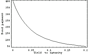
This graph represents the payment-yield relationship for the bond with a 10% coupon rate.
In[15]:=Plot[p[.10, y], {y, 0, .20}, FrameLabel -> label1];
We can easily combine the payment-yield graphs for different coupon rates. Here the coupon rates are 0% (a zero-coupon bond), 7%, and 14%.
In[16]:=Plot[{p[.0, x], p[.07, x], p[.14, x]}, {x, 0, .20},
FrameLabel -> label1];

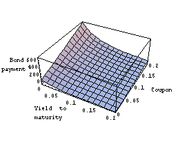
Here is the three-dimensional graph of the bond payment p[c, y] as a function of the coupon rate c and yield to maturity y. The rest of the parameters are held constant.
In[17]:=Plot3D[p[c, y], {y, 0, .20}, {c, 0, .20},
AxesLabel -> {"Yield to \nmaturity ",
" Coupon", " Bond\npayment"}];
We define a function representing the bond payment as a function of the bond object and yield to maturity.
In[18]:=bp[bond_Bond, x_] := Payment[bond, settlement1, x] /. USDollar -> 1;
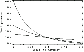
We can compare the payment-yield curves for bond3, bond10, and bond30.
In[19]:=Plot[{bp[bond3, x], bp[bond10, x], bp[bond30, x]},
{x, 0, .2}, FrameLabel -> label1];
It is interesting to look at the bond payment as a function of the length of time between the settlement and maturity.
Let abc be a bond that pays semiannual interest and matures on September 15, 2003. The redemption value is 100 units and the coupon rate is c.
In[20]:=abc = Bond[{c, {9, 15, 2023}, 100, 2}]
Out[20]=
We assume a 7% yield to maturity. We create a table of bond payments for different times to maturity.
In[21]:=p[c_] = Table[{t, Payment[abc, {9, 15, 1993 + t}, 7/100]}, {t, 0, 30}];
Here is another label.
In[22]:=label2 = {"Time in years", "Bond payment"};
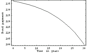
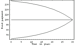
For a 10% coupon rate, abc is a premium bond. Its payment decreases over time.
In[23]:=graph1 = ListPlot[p[10 Percent],
PlotJoined -> True, FrameLabel -> label2];
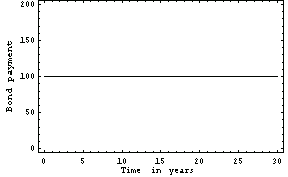
For a 7% coupon rate, abc is a par bond. Its payment does not change over time.
In[24]:=graph2 = ListPlot[p[7 Percent],
PlotJoined -> True, FrameLabel -> label2];
For a 3% coupon rate, abc is a discount bond. Its payment increases over time.
In[25]:=graph3 = ListPlot[p[4 Percent],
PlotJoined -> True, FrameLabel -> label2];

We can combine these three graphs.
In[26]:=Show[graph1, graph2, graph3];
Here is a second settlement date.
In[27]:=settlement2 = {12, 15, 1993};
Here is the accrued interest for the bonds. It is the same for all three because their coupon rates and their next coupon payment days are identical.
In[28]:=AccruedInterest[bond3, settlement2]
Out[28]=
In[29]:=AccruedInterest[bond10, settlement2]
Out[29]=
In[30]:=AccruedInterest[bond30, settlement2]
Out[30]=
This 7.5% U.S. Treasury bond pays 100 units at maturity (February 15, 1994). Here is the accrued interest on January 2, 1990.
In[31]:=AccruedInterest[Bond[{.075 , {2, 15, 1994}, 100, 2}], {1, 2, 1990}]
Out[31]=
Here are the values of bond3, bond10, and bond30.
In[32]:=Value[bond3, settlement1, .12]
Out[32]=
In[33]:=Value[bond10, settlement1, .12]
Out[33]=
In[34]:=Value[bond30, settlement1, .12]
Out[34]=
A synonym for Value is FullPayment. Here is the full bond payment of a 10% U.S. Treasury bond that matures on February 15, 1994. The settlement day is January 20, 1990 and the required yield is 6%.
In[35]:=FullPayment[Bond[{.10, {2, 15, 1994}, 100, 2}],
{1, 20, 1990}, .06]
Out[35]=
Here are the full payments of bond3, bond10, and bond30.
In[36]:=FullPayment[bond3, settlement2, .12]
Out[36]=
In[37]:=FullPayment[bond10, settlement2, .12]
Out[37]=
In[38]:=FullPayment[bond30, settlement2, .12]
Out[38]=


Additional bond function.
The yield to maturity (or internal rate of return) is the yield that would be earned if the bond were purchased at the current market price and held until maturity. It is a solution for  of the equation of the equation

Here is the bond payment for bond3 assuming a 12.5% interest rate.
In[39]:=Payment[bond3, settlement1, .125]
Out[39]=
Now we compute the yield to maturity using this payment as the price. We get 0.125, as expected.
In[40]:=YieldToMaturity[bond3, %, settlement1]
Out[40]=
Here is the payment for bond10 assuming a 6.75% interest rate.
In[41]:=Payment[bond10, settlement2, .0675]
Out[41]=
Taking the price of the bond to be this payment, we get 0.0675, again as expected.
In[42]:=YieldToMaturity[bond10, %, settlement2]
Out[42]=
Bond prices are often expressed in thirty-seconds, and coupons in eighths. For instance, you could find a bond with a price of 101:13 in The Wall Street Journal. This means  . .
This calculates the yield to maturity of a  % bond that pays semiannually and matures on September 15, 1995. The redemption value is 100 units, and its price is % bond that pays semiannually and matures on September 15, 1995. The redemption value is 100 units, and its price is  . .
In[43]:=YieldToMaturity[Bond[{(10 + 3/8) Percent, {9, 15, 1995},
100, 2}], 101 + 13/32 , {12, 15, 1993}]
Out[43]=


Sensitivity measures functions.
The Macaulay duration is the weighted average maturity of a bond's cash flows. The present values of the cash flows are the weights. It is the time to maturity of an equivalent zero-coupon bond. The Macaulay duration is also a measure of the sensitivity of a bond's price to changes in interest rates. Furthermore, the duration varies with the interest rates. The convexity is a measure of the sensitivity of the duration to interest rates changes. It is the slope of the price-yield curve of a bond.
A 14% Treasury bond matures on September 15, 1996. The yield to maturity of the bond is 15%. We calculate the Macaulay duration of the bond on July 15, 1993 in half-years.
In[44]:=Duration[Bond[{.14, {9, 15, 1996}, 1000, 2}],
{9, 15, 1993}, .15]
Out[44]=
The result is in periods. If we want it in years, we have to divide by the bond's frequency.
In[45]:=%/2
Out[45]=
We compute the durations of bond3, bond10, and bond30 on December 15, 1993 assuming a 12% yield to maturity.
In[46]:=Duration[bond3, settlement2, .12]
Out[46]=
In[47]:=Duration[bond10, settlement2, .12]
Out[47]=
In[48]:=Duration[bond30, settlement2, .12]
Out[48]=
We define bd[x, c] to be the duration in years of an x-year bond with the coupon rate c.
In[49]:=bd[x_Integer?Positive, c_] := Duration[Bond[{c,
{9, 15, 1993 + x}, 100, 2}], {9, 15, 1993}, .07] / 2;
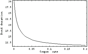
Here is the relationship between the duration and the coupon rate for a 30-year bond. The duration is more sensitive to coupon changes for lower coupon rates than for higher ones.
In[50]:=Plot[bd[30, c], {c, 0, .20},
FrameLabel -> {"Coupon rate", "Bond duration"}];
This shows the relationship between the various maturity issues. The duration is more sensitive to coupon changes for long terms to maturity than for short ones.
In[51]:=Plot[{bd[3, c], bd[10, c], bd[30, c]}, {c, 0, .20},
FrameLabel -> {"Coupon rate", "Bond duration"}];

Here we compute the convexity (in periods) for a 5-year, 14% coupon bond selling to yield 10%.
In[52]:=Convexity[Bond[{.14, {9, 15, 1998}, 1000, 2}],
settlement1, .10]
Out[52]=
The result returned by Convexity is in periods squared. So if we want to have the result in years squared we have to divide by the bond's frequency squared. This is the previous result in years squared.
In[53]:=% / 2^2
Out[53]=
Here we compute the convexity (in periods squared) for a 10-year, 8% coupon bond selling to yield 10%.
In[54]:=Convexity[Bond[{.8, {9, 15, 2003}, 1000, 2}], settlement1, .10]
Out[54]=


Auxiliary functions.
We define a third settlement date.
In[55]:=settlement3 = {8, 29, 1993};
Here is the date of the third coupon payment counted backward from maturity.
In[56]:=CouponPaymentDate[bond10, 3]
Out[56]=
This is the number of coupon payments between August 29, 1993 and the maturity of bond10.
In[57]:=n = NumberOfCouponPayments[bond3, settlement3]
Out[57]=
We can find the dates of all the coupon payments of bond3 after the settlement date.
In[58]:=tab = Table[CouponPaymentDate[bond3, k], {k, 1, n}];
Here we display them in a table.
In[59]:=TableForm[tab,
TableHeadings -> {Range[7], {"M", " D", " Y\n"}}]
Out[59]//TableForm=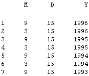
We can generate the dates of the cash flows for a given bond and settlement directly.
In[60]:=CashFlowsDates[bond3, {9, 30, 1993}] // ColumnForm
Out[60]=
|