|
Interest Rates
Flat Rates
The notion that money has a time value is one of the basic concepts in the analysis of any financial instrument. From the borrower's point of view, interest is the price of money. To an investor, interest is the compensation, or enticement, for deferring consumption to a future period. The interest rate is the market clearing price of money.
The simplest possible model of interest rates is the flat rate. Simple interest is the amount earned on the principal without allowing for interest on interest. If the interest earned is automatically reinvested we have compound interest.
This loads the InterestRates subpackage. We don't need to do this if we previously loaded Finance`.
In[1]:=<< Finance`InterestRates`


Basis interest rates functions.
We can use the units USDollar, Year, Day, etc. We have to specify how many days are in a year because the day count basis is not predefined.
A bank accepts a $100,000 deposit to mature in 300 days and will pay 7.26% per annum (p.a.) on the deposit. Here is the calculation of the future value of the deposit.
In[2]:=fv = FutureValue[100000 USDollar, 7.26 Percent/Year,
1/Year, 300 Day] /. Day -> 1/365 Year
Out[2]=
As expected, the present value of the above future value is $100,000.
In[3]:=PresentValue[fv, 7.26 Percent/Year, 1/Year, 300 Day] /.
Day -> 1/365 Year
Out[3]=
Suppose now that the interest rate is computed on the "30/360" day count basis.
In[4]:=FutureValue[100000 USDollar, 7.26 Percent/Year, 1/Year,
300 Day] /. Day -> 1/360 Year
Out[4]=

Option for FutureValue and PresentValue.
In finance we often want to display results with a fixed accuracy. There are two pre-defined functions to display results with an accuracy of two or three decimal places.
In[5]:=TwoPlaces[987654321.123456789]
Out[5]//NumberForm=
In[6]:=ThreePlaces[987654321.123456789]
Out[6]//NumberForm=
A bank accepts a $500,000 deposit to mature in three years and will pay 14.79% p.a. on the deposit. This is the future value of this deposit.
In[7]:=compound = FutureValue[500000 USDollar, 14.79 Percent /
Year, 1 / Year, 3 Year]
Out[7]=
Interest rates are compounded by default. For simple interest rates we have to set the option Compounded to False.
In[8]:=simple = FutureValue[500000 USDollar, 14.79 Percent /
Year, 1 / Year, 3 Year, Compounded -> False]
Out[8]=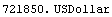
This is the interest-on-interest in this case.
In[9]:=compound - simple // TwoPlaces
Out[9]=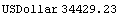
Compound interest rates are quoted in terms of nominal percentage p.a. yields. The effective per annum interest rate depends on the frequency with which the interest is assumed to compound during each year. If the nominal rate is  and the interest rate is paid and the interest rate is paid  times per year, the interest rate per period is times per year, the interest rate per period is  and the effective interest rate p.a. is and the effective interest rate p.a. is  . .
Here is a quarterly paid nominal interest rate equivalent to the nominal rate of 10% p.a. paid semiannually.
In[10]:=NominalRate[10 Percent/Year, 2/Year, 4/Year]
Out[10]=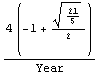
This is a numerical approximation.
In[11]:=N[%]
Out[11]=
The nominal rate for a unit of frequency is the effective rate for that frequency. Here is the calculation of the effective annual rate for a 10% nominal rate paid semiannually.
In[12]:=NominalRate[10 Percent/Year, 2/Year, 1/Year] // N
Out[12]=
Term Structure of Interest Rates
The relation between promised security yields and security maturities is referred to as the term structure of interest rates. This is a more sophisticated approach to security valuation than the flat interest rates model. We can represent interest rates in a number of equivalent ways.


Interest rates objects.

Option for SpotRates, ForwardRates, and DiscountFactors objects.
The Finance Pack supports spot rates, forward rates, and discount factors. Any of these can be used to define an interest rates object. Once an interest rates object is defined, in some sense it becomes independent of its original representation. This means that once we define the interest rates object we can get any other representation immediately. We will discuss this further in Section 3.6. We can manipulate an object to extract its class, description, or options.
Spot Rates
A spot rate is the interest rate on a pure discount bond with a specified maturity. In other words, it is the interest rate on a single cash flow received at a future time. Spot rates are represented by a list of ordered pairs. The first element of each pair is the time from a given initial date. The second element is the rate for the corresponding period. The pairs must be ordered so that the time intervals increase.
Here is an example of a spot rates object. Usually we do not need to specify the initial date, but we can do so with the option InitialDate, which has the default value Automatic.
In[13]:=spot0 = SpotRates[{{1, 0.0814},
{2, 0.0904},
{3, 0.0951},
{5, 0.1002},
{7, 0.1050},
{10, 0.1066},
{30, 0.1078}},
InitialDate->{7, 30, 1985}];
We can use ListPlot to plot the yield curve.
In[14]:=ListPlot[First[%], PlotJoined->True];
Suppose the spot rates in the above example are not given in the right order. We can get the correct order in a straightforward way with Sort.
In[15]:=Sort[{{30, 0.1078},
{2, 0.0904},
{5, 0.1002},
{3, 0.0951},
{1, 0.0814},
{7, 0.1050},
{10, 0.1066}}]
Out[15]=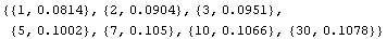
We can use Sort inside the definition of a spot rates object.
In[16]:=spot1 = SpotRates[Sort[
{{30, 0.1078},
{2, 0.0904},
{5, 0.1002},
{3, 0.0951},
{1, 0.0814},
{7, 0.1050},
{10, 0.1066}}],
InitialDate->{7, 30, 1985}]
Out[16]=
Note that we can use units. In this example, the time intervals are expressed in years, but we can also use days, months, bimonths, quarters, or periods.
In[17]:=spot2 = SpotRates[
{{1 Year, 16.97 Percent / Year},
{2 Year, 16.73 Percent / Year},
{3 Year, 16.33 Percent / Year},
{5 Year, 16.11 Percent / Year},
{7 Year, 15.71 Percent / Year},
{10 Year, 15.41 Percent / Year},
{30 Year, 14.78 Percent / Year}},
InitialDate->{8, 31, 1981}];
Here is another example of a spot rates object.
In[18]:=spot3 = SpotRates[{{1, 0.0691},
{2, 0.0764},
{3, 0.0789},
{5, 0.0816},
{7, 0.0844},
{10, 0.0861},
{30, 0.0885}},
InitialDate->{7, 29, 1987}];
Mathematica allows you to use symbols as well as numbers.
In[19]:=spot4 = SpotRates[{s1, s2, s3, s4}]
Out[19]=
The function Head can be used to check the type of an object.
In[20]:=Head[spot1]
Out[20]=
This extracts the description.
In[21]:=First[spot4]
Out[21]=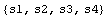
This shows how the options are set.
In[22]:=Options[spot3]
Out[22]=
We load the file spots.m. It contains spot rates named spot[i], where i = 1, 2, ... , 8.
In[23]:=Get["Finance`Data`spots`"]
Here is the first of these objects.
In[24]:=spot[1]
Out[24]=
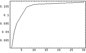
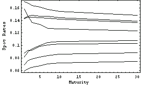
The yield curve is the graphical representation of a spot rates object. This function will create a yield curve without displaying it.
In[25]:=yieldcurve[i_] := ListPlot[Evaluate[First[spot[i]]],
PlotJoined -> True, DisplayFunction -> Identity];
Here we display all eight yield curves. This graph proves that in this case the flat interest rates model is not a good approximation to the true term structure.
In[26]:=Show[Table[yieldcurve[i], {i, 8}],
DisplayFunction -> $DisplayFunction,
FrameLabel -> {"Maturity", "Spot Rates"}];
Forward Rates
A forward rate is a yield on the margin between two successive spot rates. It is the future interest rate implicit in the yield curve. Forward rates are represented like spot rates except that the first number of each pair represents the length of the consecutive time interval instead of the time from a given date. The second element of each pair is the forward rate for that period.
Here we define a forward rates object.
In[27]:=forward1 = ForwardRates[
{{1, 0.088300},
{1, 0.096716},
{1, 0.093400},
{2, 0.107610},
{2, 0.106419},
{3, 0.106242},
{20, 0.104300}},
InitialDate->{5, 30, 1980}];
Discount Factors
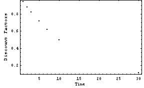
Discount interest factors are multipliers that translate the future value of an investment into its equivalent present value. Again, discount factors are represented by a list of ordered pairs. As with spot rates, the first element of each pair represents the time from a given date. The second element is the actual discount factor. The pairs must be sorted in order of increasing time.
This defines a discount factors object.
In[28]:=discount1 = DiscountFactors[
{{1, 0.943841},
{2, 0.884148},
{3, 0.826451},
{5, 0.719350},
{7, 0.619095},
{10, 0.49755},
{30, 0.11454}},
InitialDate -> {12, 31, 1986}];
And here is the graph of the discount factors.
In[29]:=ListPlot[First[discount1],
FrameLabel -> {"Time", "Discount Factors"}];
Assuming that interest rates are piecewise linear functions of time, we can compute the interpolated discount factors over the given time range.


InterpolatedDiscountFactors function.
This gives the discount factors for 4 and 8 years from a given time.
In[30]:=InterpolatedDiscountFactors[discount1, {4, 8}]
Out[30]=
This gives the largest time interval in the discount1 object.
In[31]:=max = Part[discount1, 1, -1, 1]
Out[31]=
We can produce the interpolated discount factors for all the intervals and define a new discount rates object.
In[32]:=discount2 = DiscountFactors[
InterpolatedDiscountFactors[discount1,
Range[max]]]
Out[32]=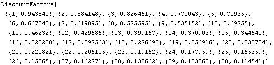
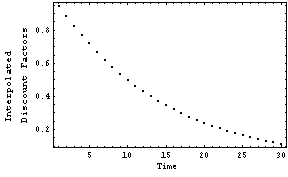
This is the graph of the interpolated discount factors.
In[33]:=ListPlot[First[discount2],
FrameLabel -> {"Time",
"Interpolated\nDiscount Factors"}];
We define a forward rates object.
In[34]:=forward2 = ForwardRates[
{{1, 0.1434},
{1, 0.149809},
{1, 0.150204},
{2, 0.144553},
{2, 0.14685},
{3, 0.139283},
{20, 0.136459}},
InitialDate -> {6, 30, 1982}]
Out[34]=
This little function computes the sum of the intervals of a forward rates object.
In[35]:=intervalSum[object_ForwardRates] :=
Apply[Plus, First[Transpose[First[object]]]]
You can use any of our interest rates objects to calculate the interpolated discount factors. Here we are using forward rates.
In[36]:=InterpolatedDiscountFactors[forward2,
Range[intervalSum[forward2]]]
Out[36]=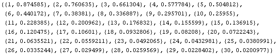
Of course, you can write a more sophisticated version of InterpolatedDiscountFactors; this one assumes that interest rates are piecewise constant over time.
Interest Rates Conversions
SpotRates, ForwardRates, and DiscountFactors are polymorphic in that they are interest rates objects as well as conversion functions. The way that interest rates are related to their representation is analogous to how a geometric figure is related to a coordinate system. You can define a set of points using one coordinate system and then you can describe the points using any other coordinate system. In a sense our object becomes independent of its initial representation. This is true for any of the interest rates representations.
Suppose we have defined an interest rates object using spot rates. We can now use any of the representations.
In[37]:=spot = SpotRates[
{{1, 14.30 Percent},
{2, 14.52 Percent},
{3, 14.52 Percent},
{5, 14.39 Percent},
{7, 14.37 Percent},
{10, 14.18 Percent},
{30, 13.68 Percent}},
InitialDate -> {3, 31, 1982}];
Here is the discount factors representation of the object originally defined using spot rates.
In[38]:=DiscountFactors[spot]
Out[38]=
Here is its forward rates representation.
In[39]:=ForwardRates[spot]
Out[39]=
Of course, the spot rates representation of spot is the one we started with.
In[40]:=SpotRates[spot]
Out[40]=
The "round trip" does not change the original object.
In[41]:=SpotRates[ForwardRates[DiscountFactors[spot]]] == spot
Out[41]=
We can also work with symbols.
In[42]:=SpotRates[ForwardRates[{f1, f2, f3, f4}]]
Out[42]=
Simple Representation of Interest Rates
The representation of interest rates can be simplified if the time intervals are 1, 2, 3, 4 ... in some given unit. We no longer need a list of pairs because the first element of each pair is simply the position of the pair in the list. It is enough to know just the list of actual interest rates. Our package supports this representation.
This is the simple representation of a spot rates object.
In[43]:=spot0 = SpotRates[
{0.08927,
0.08743,
0.08886,
0.08701,
0.08726,
0.09137,
0.09386,
0.08997,
0.08967,
0.09152}]
Out[43]=
This converts spot0 to the equivalent discount0.
In[44]:=discount0 = DiscountFactors[spot0]
Out[44]=
This converts spot0 to the equivalent forward0.
In[45]:=forward0 = ForwardRates[spot0]
Out[45]=
Again the "round trip" does not change the original object.
In[46]:=SpotRates[ForwardRates[DiscountFactors[spot0]]] == spot0
Out[46]=
All the representations are equivalent.
In[47]:=forward0 == ForwardRates[discount0]
Out[47]=
In[48]:=spot0 == SpotRates[forward0]
Out[48]=
The time intervals for a discount rates object do not necessarily have to be uniform. For example, to calculate the present value, it is only required that time intervals for discount factors match those of the corresponding cash flows. However, converting from one simple representation to another will cause errors.
|