|
3.9.5 RootLocusPlot
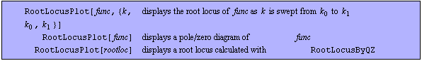
Command structure of RootLocusPlot.
RootLocusPlot displays a root locus plot of a transfer function  , where , where  denotes a real-valued parameter. A root locus plot shows the trajectories of the poles and zeros of denotes a real-valued parameter. A root locus plot shows the trajectories of the poles and zeros of  in the complex plane as in the complex plane as  varies from varies from  to to  . RootLocusPlot can also be used to produce a pole/zero diagram of transfer function . RootLocusPlot can also be used to produce a pole/zero diagram of transfer function  without parameters as well as to display root loci calculated with RootLocusByQZ. without parameters as well as to display root loci calculated with RootLocusByQZ.
By default, RootLocusPlot chooses a logarithmic representation of the complex plane for better visualization of widely separated poles and zeros. However, as logarithmic scaling is inappropriate for coordinates near the axes, the regions around the axes are scaled semi-logarithmically, and the region around the origin is scaled linearly. RootLocusPlot marks the linearly scaled region with a gray background. The semi-logarithmic regions are the regions above and below as well as to the left and the right of the linear region.
You can customize the appearance of root locus plots with the following options. In addition, RootLocusPlot inherits many options from Graphics. Both the options which are specific to RootLocusPlot as well as the inherited options can be set with SetOptions[RootLocusPlot, opts].
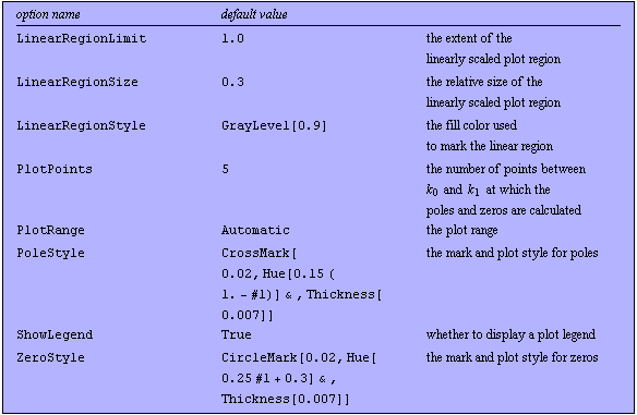
Options for RootLocusPlot.
See also: PolesAndZerosByQZ, RootLocusByQZ.
Options Description
A detailed description of all options that are specific to RootLocusPlot or are used in a non-standard way is given below in alphabetical order:
LinearRegionLimit
With LinearRegionLimit -> value, you can specify the extent of the linearly scaled plot region around the origin. For example, the setting LinearRegionLimit -> 100 causes the region where  and and  to be scaled linearly. LinearRegionLimit -> Infinity turns off logarithmic scaling. to be scaled linearly. LinearRegionLimit -> Infinity turns off logarithmic scaling.
LinearRegionSize
LinearRegionSize -> size specifies the percentage of the total plot area occupied by the linear region. The option value size must be a real number between  and and  . .
LinearRegionStyle
With LinearRegionStyle -> style, you can specify the fill color RootLocusPlot uses for the linearly scaled region.
PlotRange
The meaning of the PlotRange option is the same as for other Mathematica graphics functions, but the option has slightly different formats.
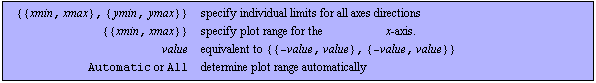
Values for the PlotRange option.
PoleStyle
With the option PoleStyle -> style, you can change the appearance of the symbol RootLocusPlot uses to mark poles. The following styles are available:
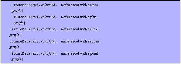
Styles for the PoleStyle and ZeroStyle options.
In the above table, size denotes the size of a root marker in scaled coordinates, colorfunc a pure function that returns a color value for an argument between 0 and 1, and grstyle an additional list of graphics styles for the root marker. The color function is used to visualize the parameter dependency of the root.
ZeroStyle
With the option ZeroStyle -> style, you can change the appearance of the symbol RootLocusPlot uses to mark zeros. For a list of available styles see the description of the PoleStyle option.
Examples
Load Analog Insydes.
In[1]:= <<AnalogInsydes`
Define a transfer function  . .
In[2]:= Ha[s_, a_] := (a + 2*s + s^2)/(10 + 3*a*s + 4*s^2 + s^3)
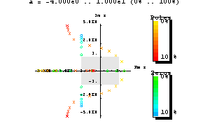
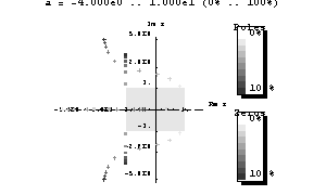
Display a root locus plot of  as as  is swept from is swept from  to to  . .
In[3]:= RootLocusPlot[Ha[s, a], {a, -4, 10}, PlotPoints -> 10]
Out[3]= 
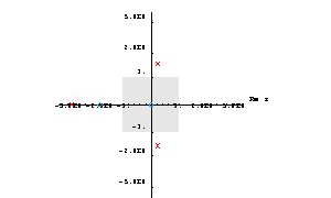
Display the pole/zero distribution of  for for  . .
In[4]:= RootLocusPlot[Ha[s, 0], PlotRange -> 6]
Out[4]= 
Change boundaries, plot size, and color of the linear region.
In[5]:= RootLocusPlot[Ha[s, a], {a, -4, 10},
PlotPoints -> 10, LinearRegionLimit -> 4.0,
LinearRegionSize -> 0.8,
LinearRegionStyle -> GrayLevel[0.95]]
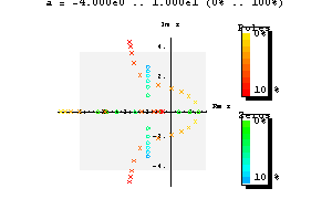
Out[5]= 
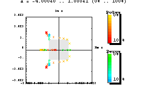
Set equal plot limits for all axes directions.
In[6]:= RootLocusPlot[Ha[s, a], {a, -4, 10},
PlotPoints -> 10, PlotRange -> 100, Frame -> True]
Out[6]= 
Change the style for pole and zero markers.
In[7]:= RootLocusPlot[Ha[s, a], {a, -4, 10},
PlotPoints -> 10,
PoleStyle -> PlusMark[0.02,
GrayLevel[1-0.8*#]&, Thickness[0.005]],
ZeroStyle -> SquareMark[0.02,
GrayLevel[1-0.8*#]&, Thickness[0.005]]]
Out[7]= 
|