|
2.10.2 Analyzing a Square Root Function Block
In this section the application of the nonlinear simplification functions is demonstrated on an example. Figure 10.1 shows the schematic of a nonlinear square root function block consisting of four bipolar transistors.
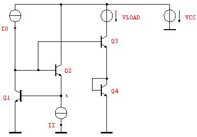
Figure 10.1: Square root function block
The input is given by the current source II and the voltage source VLOAD, the output is given by the current through the voltage source VLOAD. Using the nonlinear approximation routines we want to generate a symbolic expression for the static input output behavior of the circuit.
Importing Numerical Data
In PSpice the numerical simulation is performed as a DC sweep on ii and vload. The corresponding part of the .cir-file looks as follows:
.op
.dc ii 0.0 0.001 0.00001 vload 0 3.5 0.875
.probe/csdf
.options numdgt=8
As a first step we import the numerical simulation data calculated with PSpice into Mathematica using ReadSimulationData.
In[1]:= <<AnalogInsydes`
In[2]:= data = ReadSimulationData[
"AnalogInsydes/DemoFiles/Sqrt.txt",
Simulator -> "PSpice"]
Out[2]= 
ReadSimulationData returns the two-dimensional sweep data as a list of lists of one-dimensional interpolating functions as described in Section 3.7.1. To transform the data into a list of two-dimensional interpolating functions we can use the command ConvertDataTo2D. In the following step we extract the interpolating function corresponding to the output value I(VLOAD) and assign it to the function ivloadPSpice.
In[3]:= data2d = ConvertDataTo2D[data]
Out[3]= 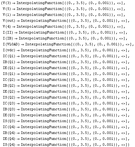
In[4]:= ivloadPSpice[VLOAD_, II_] =
"I(VLOAD)"[VLOAD, II] /. data2d
Out[4]= 
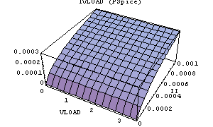
The interpolating function ivloadPSpice can now be plotted in a three-dimensional plot:
In[5]:= Plot3D[ivloadPSpice[VLOAD, II],
{VLOAD, 0., 3.5}, {II, 0., 0.001},
AxesLabel -> {"VLOAD", "II", ""},
PlotLabel -> "IVLOAD (PSpice)"]
Out[5]= 
Equation Setup
In the next step the equation system has to be set up. For this we import the PSpice .cir-file and convert it into an Analog Insydes Circuit object using the command ReadNetlist.
In[6]:= netlist = ReadNetlist[
"AnalogInsydes/DemoFiles/Sqrt.cir",
Simulator -> "PSpice"];
DisplayForm[netlist]
Out[7]//DisplayForm= 
Afterwards, we set up a symbolic DC equation system using the modified nodal formulation. Since we are not interested in temperature effects, we instruct CircuitEquations to replace TEMP, TNOM, the elementary charge $q, and Boltzmann's constant $k by their numerical values.
In[7]:= mnaFull = CircuitEquations[netlist,
AnalysisMode -> DC, ElementValues -> Symbolic,
Value -> {"*" -> {TEMP, TNOM, $q, $k}}]
Out[8]= 
In[8]:= GetVariables[mnaFull]
Out[9]= 
In[9]:= GetParameters[mnaFull]
Out[10]= 
Numerical Reference Calculation
Using NDAESolve we now perform the same numerical simulation as in PSpice, transform the result again into a two-dimensional interpolating function, and plot it in a three-dimensional plot.
In[10]:= data = NDAESolve[mnaFull,
{II, 0.0, 0.001}, {VLOAD, 0., 3.5, 0.5}];
In[11]:= data2d = ConvertDataTo2D[data];
In[12]:= ivload[VLOAD_, II_] = I$VLOAD[VLOAD, II] /. data2d
Out[13]= 
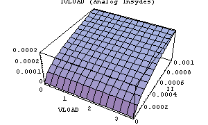
In[13]:= Plot3D[ivload[VLOAD, II],
{VLOAD, 0., 3.5}, {II, 0., 0.001},
AxesLabel -> {"VLOAD", "II", ""},
PlotLabel -> "IVLOAD (Analog Insydes)"]
Out[14]= 
Model Validation
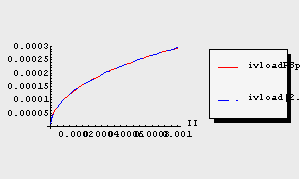
One key step is now to check if the numerical simulation in Analog Insydes is identical to the result of the PSpice simulation, i.e. to check if we have chosen appropriate transistor models. This can for example be done by comparing the graphical output. We choose some arbitrary value for VLOAD and plot both output values in one graph sweeping II. The plot shows that both curves are identical (for this value of VLOAD). Alternatively, we can calculate the maximum difference of both output values evaluated on a uniform grid. The result shows that the deviation is of order  . .
In[14]:= TransientPlot[{ivloadPSpice[2., II], ivload[2., II]},
{II, 0., 0.001}]
Out[15]= 
In[15]:= Max @ Map[Abs[Apply[ivload,#] - Apply[ivloadPSpice,#]] &,
Flatten[Table[{VLOAD, II},
{VLOAD, 0., 3.5, 0.1}, {II,0., 0.001, 0.000025}], 1]]
Out[16]= 
Starting Nonlinear Simplifications
Now that we have ensured to use the same equation system as PSpice does, we can proceed with the nonlinear simplification routines. The task is to generate a simplified static equation system which has the same input-output behavior as the original system mnaFull. To get an impression of the complexity of the original system, we use the command Statistics.
In[16]:= Statistics[mnaFull]

Compressing Equations
In a first step we eliminate irrelevant variables using the function CompressNonlinearEquations. The argument {I$VLOAD} to CompressNonlinearEquations assures that our variable of interest is not eliminated from the equation system. Eliminating variables is a mathematically exact operation, thus no error calculation is needed. As in our example, this usually reduces the number of equations drastically (but not necessarily the number of terms) and is therefore recommended as the first step in the simplification procedure.
In[17]:= step1 = CompressNonlinearEquations[mnaFull, {I$VLOAD}]
Out[18]= 
In[18]:= Statistics[step1]

Preparing Approximation Routines
To further reduce the complexity of the DAE system we now cancel terms in the equations. Since this operation alters the output of the system, numerical control simulations have to be applied to check the current error. We use NonlinearSetup to prepare the DAEObject for the following simplification steps. Since we are dealing with a static equation system, we choose the DT analysis mode for error checking, specifying sweep ranges for both input values VLOAD and II. NonlinearSetup performs a numerical reference simulation and stores the result in the returned DAEObject. These numerical values are used automatically to calculate the error in subsequent simplification steps.
In[19]:= step2 = NonlinearSetup[step1, {II, VLOAD}, {I$VLOAD},
DT -> {Range ->
{{VLOAD, 0., 3.5, 0.5}, {II, 0., 0.001, 0.0002}} }]
Out[20]= 
Cancelling Terms
Once we have set up the DAE system we call CancelTerms where we specify an error bound for the output variable. CancelTerms then deletes terms in the equation system using this error bound. Afterwards we again use Statistics to inspect the complexity reduction achieved by CancelTerms.
In[20]:= step3 = CancelTerms[step2, {DT -> {I$VLOAD -> 25.*^-6}}]
Out[21]= 
In[21]:= Statistics[step3]

Note that CancelTerms reduces the number of terms drastically.
Compressing Equations again
Deletion of terms changes the equations in such a way that it is often possible to further solve equations for some variables. Thus, we can again try to eliminate variables using CompressNonlinearEquations. Here, two more equations can be removed from the system. Note that CompressNonlinearEquations automatically retrieves the settings made by NonlinearSetup, so there is no need to specify the variable of interest I$VLOAD as a second argument. Afterwards we drop those parameters from the design point which no longer appear in the equation system using UpdateDesignPoint.
In[22]:= step4 = CompressNonlinearEquations[step3]
Out[23]= 
In[23]:= Statistics[step4]

In[24]:= step5 = UpdateDesignPoint[step4]
Out[25]= 
In[25]:= step5 // DisplayForm
Out[26]//DisplayForm= 
Looking at the simplified DAE system one can see that the parameter VLOAD disappeared from the equations. The three-dimensional plot of the output from the beginning shows that the output does not depend on VLOAD, thus the simplification procedure automatically removes this parameter from the equation system.
Validating the Result
Now we can compare the output of the simplified system step5 with the output of the original system. Since VLOAD no longer appears in the DAE system, we no longer need to perform a multi-dimensional parametric sweep of NDAESolve. A single sweep on II suffices, resulting in a one-dimensional interpolating function.
In[26]:= data = NDAESolve[step5, {II, 0., 0.001}];
In[27]:= ivloadSimp[II_] = I$VLOAD[II] /. First @ data
Out[28]= 
In[28]:= Plot3D[ivloadSimp[II],
{VLOAD, 0., 3.5}, {II, 0., 0.001},
AxesLabel -> {"VLOAD", "II", ""},
PlotLabel -> "IVLOAD (simplified system)"]

Out[29]= 
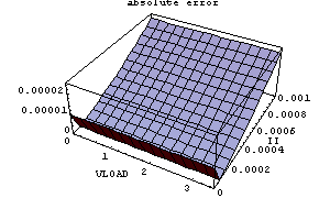
To show that the requested error bound is met, we plot the deviation of the output comparing the original and the simplified system (note the plot range).
In[29]:= Plot3D[Abs[ivloadSimp[II]-ivload[VLOAD, II]],
{VLOAD, 0., 3.5}, {II, 0., 0.001},
PlotRange -> {0, 25.*^-6},
AxesLabel -> {"VLOAD", "II", ""},
PlotLabel -> "absolute error"]
Out[30]= 
Further Postprocessing
In the final step we further reduce the complexity of the equation system by applying some standard Mathematica functions to manipulate the equations symbolically. In this example it is possible to solve the equations for the output variable I$VLOAD symbolically yielding an explicit formula describing the input-output behavior.
In[30]:= eqs = GetEquations[step5];
In[31]:= eqs2 = Eliminate[eqs, {V$3, V$4, V$5}]

Out[32]= 
In[32]:= Solve[Map[Exp, eqs2], I$VLOAD]
Out[33]= 
From the result it can be seen that the output current I$VLOAD depends on the square root of the input current II and that it is independent of the input voltage VLOAD.
|