2.6.5 Multi-Dimensional Models

The Ebers-Moll Transistor Model

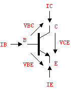
The procedure for modeling one-dimensional nonlinear element characteristics can be easily extended to the multi-dimensional case. Let's demonstrate multi-dimensional device modeling on a practical example by defining nonlinear DC models for a bipolar junction transistor (see Figure 6.4).

Figure 6.4: NPN transistor

Our considerations will be based on the BJT model introduced by Ebers and Moll which expresses the relations between the transistor currents and voltages , , , and as

In these equations, the parameter represents the transport saturation current, and denote the large-signal reverse and forward current gains of the common base configuration, and designates the thermal voltage. In integrated circuit design, the saturation current is usually expressed as the product of the transport saturation current density , which is a process parameter, and the emitter area , which is a design parameter:

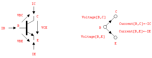
The remaining two unknown voltages and currents at the transistor's terminals, and can be computed from KCL and KVL (see Figure 6.5) as

Figure 6.5: NPN transistor and corresponding ABM port branch definition

In most linear applications, bipolar transistors are typically operated in the forward active region which is roughly characterized by and . Under these assumptions we can simplify the Ebers-Moll model to

because as compared to the terms involving , all other terms are smaller by several orders of magnitude.

A BJT operating in the forward active region acts as a good current amplifier from the base current  to the collector current  with the gain relationship

The parameter denotes the large-signal forward current gain in common-emitter configuration. It is often more convenient to think in terms of forward and reverse current gains with respect to the base current, i.e. and , than in terms of the model parameters and in the original Ebers-Moll equations. The relationship between and , as well as between and is given by

or, equivalently,

By making use of parameter translation rules in the model definition (see Section 2.3.7), we can let Analog Insydes compute the values for and automatically from given values for and .

Implementation of Nonlinear DC Transistor Models

With the above background information on transistor models we are now ready to define a large-signal BJT model for DC circuit analysis. We start by implementing a global DC model for an NPN transistor using the unsimplified device equations after Ebers and Moll from the previous subsection.

Name -> NPNBJT,

Selector -> EbersMoll,

Scope -> Global,

Ports -> {C, B, E},

Let's decide that we do not want to characterize a transistor by the Ebers-Moll model parameters Is, alphaf, alphar, and Vt but want to use the parameters Js, Area, betaf, betar, and Temperature instead. We do not need to rewrite the model equations if we specify translation rules which translate our model parameters to those of the Ebers-Moll model. Remember that the function ThermalVoltage has already been defined in Section 2.6.2.

Parameters -> {betaf, betar, Js, Area, Global[Temperature]},

Translation ->

{alphaf -> betaf/(1+betaf), alphar -> betar/(1+betar),

Is -> Js*Area, Vt :> ThermalVoltage[Temperature]},

The Ebers-Moll equations describe the functional relations between the voltages and currents at two electrical branches, the base-collector branch and the base-emitter branch, which we use as the port branches of our model. Associated with the port branches are the variables Voltage[B, E], Current[B, E], Voltage[B, C], and Current[B, C], which must be specified as

Variables ->

{Current[B, C], Voltage[B, C],

Current[B, E], Voltage[B, E]},

in the model definition.

It remains to write the model equations in terms of the port branch variables, paying attention to the different positive reference directions assumed for the port currents as compared to and in the Ebers-Moll equations. While the latter are defined to be positive for currents flowing into the collector and emitter, positive values of Current[B, C] and Current[B, E] denote currents flowing out of these terminals. We account for this difference by changing the sign on the right-hand side of the model equations.

Definition ->

Equations[

Current[B, C] == -Is*(Exp[Voltage[B, E]/Vt] - 1)

+ Is/alphar*(Exp[Voltage[B, C]/Vt] - 1),

Current[B, E] == Is/alphaf*(Exp[Voltage[B, E]/Vt] - 1)

- Is*(Exp[Voltage[B, C]/Vt] - 1)

],

To store the transistor model in the global database we wrap the complete Model definition into a Circuit structure and expand it with ExpandSubcircuits.

In[8]:= Circuit[
Model[
Name -> NPNBJT,
Selector -> EbersMoll,
Scope -> Global,
Ports -> {C, B, E},
Parameters ->
{betaf, betar, Js, Area, Global[Temperature]},
Translation ->
{alphaf -> betaf/(1+betaf),
alphar -> betar/(1+betar),
Is -> Js*Area, Vt :> ThermalVoltage[Temperature]},
Variables ->
{Current[B, C], Voltage[B, C],
Current[B, E], Voltage[B, E]},
Definition ->
Equations[
Current[B, C] == -Is*(Exp[Voltage[B, E]/Vt] - 1)
+ Is/alphar*(Exp[Voltage[B, C]/Vt] - 1),
Current[B, E] == -Is*(Exp[Voltage[B, C]/Vt] - 1)
+ Is/alphaf*(Exp[Voltage[B, E]/Vt] - 1)
]
]
] // ExpandSubcircuits;

Similarly, we define a simplified Ebers-Moll model for transistors operating in the forward active region.

In[9]:= Circuit[
Model[
Name -> NPNBJT,
Selector -> EbersMollForwardActive,
Scope -> Global,
Ports -> {C, B, E},
Parameters -> {betaf, Js, Area, Global[Temperature]},
Translation ->
{alphaf -> betaf/(1+betaf),
Is -> Js*Area, Vt :> ThermalVoltage[Temperature]},
Variables ->
{Current[B, C], Voltage[B, C],
Current[B, E], Voltage[B, E]},
Definition ->
Equations[
Current[B, C] == -Is*(Exp[Voltage[B, E]/Vt]),
Current[B, E] == Is/alphaf*(Exp[Voltage[B, E]/Vt])
]
]
] // ExpandSubcircuits;

Both models are now stored in the global database:

In[10]:= GlobalSubcircuits[]

Out[12]=