|
2.6.6 Nonlinear DC Circuit Analysis
Calculating the Bias Point of a Transistor Circuit
Analog Insydes' nonlinear modeling capabilities and numeric equation solver allow for solving circuit analysis problems quickly and reliably without tedious and error-prone hand calculations. Let's demonstrate one such application:
Determine the operating-point currents and voltages IB, IC, VBE, VCE for the circuit shown in Figure 6.6, if (a)  and (b) and (b)  . Assume that the transistor has an emitter area of . Assume that the transistor has an emitter area of  , ,  , ,  , ,  , and that it operates at a temperature of , and that it operates at a temperature of  . The values of the supply voltage and the collector resistance are . The values of the supply voltage and the collector resistance are  and and  . .
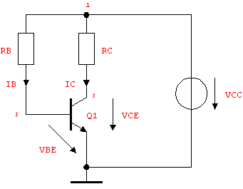
Figure 6.6: Bipolar transistor circuit
For didactic reasons we do not use ReadNetlist to automatically import the netlist, but rather write the circuit by hand. Moreover, instead of using a BJT transistor model from the predefined Analog Insydes model library, we select a suitable model from the global database which contains the two NPNBJT models defined in the previous section. By leaving the model selector unspecified, Selector -> BJTModel, we can postpone the final choice of the underlying model equations until we set up circuit equations. The option Pattern -> Impedance in the value field of RB introduces the current I$RB into the MNA equations. The current I$RB is identical to the base current IB, so we can compute the latter directly from the equations without having to determine it manually from IC and IE by KCL.
In[11]:= bjtbias =
Circuit[
Netlist[
{VCC, {1, 0}, Type -> VoltageSource,
Symbolic -> VCC, Value -> 12.},
{RB, {1, 2}, Pattern -> Impedance,
Symbolic -> RB, Value -> 500.*10^3},
{RC, {1, 3}, Symbolic -> RC, Value -> 4000.},
{Q1, {3 -> C, 2 -> B, 0 -> E},
Model -> NPNBJT, Selector -> BJTModel,
betaf -> 100., betar -> 0.2,
Js -> 6.*10^-16, Area -> 4., Temperature -> 300.}
]
]
Out[13]= 
In order to keep model complexity as low as possible, we make the initial assumption that Q1 operates in the forward active region and set up a system of symbolic static circuit equations using the simplified Ebers-Moll model by setting the options AnalysisMode -> DC and ElementValues -> Symbolic.
In[12]:= mnaeqsfa = CircuitEquations[
bjtbias /. BJTModel -> EbersMollForwardActive,
AnalysisMode -> DC, ElementValues -> Symbolic];
DisplayForm[mnaeqsfa]
Out[15]//DisplayForm= 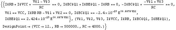
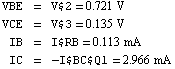
This system of equations can be solved by Analog Insydes' numerical root finding function NDAESolve, which starts from an initial guess for the values of the variables. By default, initial values of  for all unknowns are chosen which is very often close enough to ensure convergence. for all unknowns are chosen which is very often close enough to ensure convergence.
In[13]:= NDAESolve[mnaeqsfa, {t, 0}]
Out[16]= 
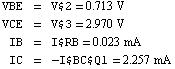
From the result we can immediately read off the operating point. We have
Next, we repeat the same calculation for  using the command UpdateDesignPoint to alter the numeric element value for RB. using the command UpdateDesignPoint to alter the numeric element value for RB.
In[14]:= mnaeqsfa = UpdateDesignPoint[mnaeqsfa, RB -> 1.*10^5];
NDAESolve[mnaeqsfa, {t, 0}]
Out[18]= 
This time, we obtain a physically nonsensical value of  for VCE which indicates that our initial assumption about the operating condition of Q1 has been violated. Indeed, for for VCE which indicates that our initial assumption about the operating condition of Q1 has been violated. Indeed, for  , Q1 operates in deep saturation. We must therefore select the full Ebers-Moll model to take these effects into account. , Q1 operates in deep saturation. We must therefore select the full Ebers-Moll model to take these effects into account.
In[15]:= mnaeqssat = CircuitEquations[
bjtbias /. BJTModel -> EbersMoll,
AnalysisMode -> DC, ElementValues -> Symbolic];
DisplayForm[mnaeqssat]
Out[20]//DisplayForm= 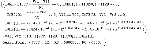
Solving these enhanced equations will now deliver a proper result for  . .
In[16]:= mnaeqssat = UpdateDesignPoint[mnaeqssat, RB -> 1.*10^5];
NDAESolve[mnaeqssat, {t, 0}]
Out[22]= 
We finally obtain:
|