Rear Suspension

Example Mechanism for
Velocity and Acceleration Functions

by Robert Beretta

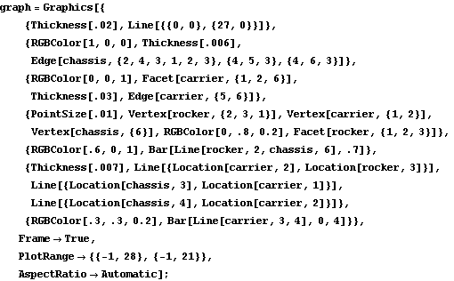
Rear Suspension Animation

Discussion

Suspension Function

This sample notebook analyzes the motion of an inboard damper rear suspension system using the MechanicalSystems kinematics package. This mechanism is used to demonstrate the use of Modeler2D's velocity and acceleration solution methods.

Suspension Model

The inboard damper rear suspension system consists of four bodies.
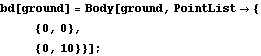
1. Ground        (black)
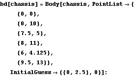
2. Chassis        (red)
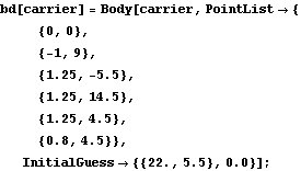
3. Wheel carrier    (blue)
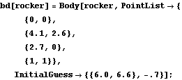
4. Rocker arm    (green)

The ground body is the earth. The input to the model is the chassis moving vertically relative to the earth. This model could have been reduced in size by making the ground body the chassis and simply moving the wheel carrier relative to the chassis, but the chosen method allows more flexibility and makes for better graphics.

The wheel carrier is attached to the chassis by two A-arms. These A-arms are not modeled as independent bodies because their function can be represented by a pair of relative-distance constraints between the chassis and the wheel carrier. These constraints simply enforce the absolute distance between two points to be equal to a constant.

The rocker arm pivots about an axis affixed to the chassis and is attached to the wheel carrier by a connecting link in tension. This connecting link is also modeled with a relative-distance constraint. The damper, or shock absorber, is connected between the other end of the rocker arm and the chassis. The damper is not actually part of the kinematic model at all, but the length of the damper as a function of wheel motion is a primary point interest for any suspension system.

Kinematic Model

Preparation

The Modeler2D package is loaded into Mathematica with the Needs command.

Bodies in a MechanicalSystems model are referenced by a positive integer body number. The following names are used to reference each of the bodies in the suspension model throughout the analysis.

Body Definitions

Body objects are defined for each of the bodies in the model. The body objects contain the coordinates of points in each body's local coordinate system. Other Mech functions can reference these local point coordinates by their positive integer point numbers. The body objects also contain initial guesses for the global coordinates of each body.

Ground

Two points are defined on the ground (body 1).
P1 and P2. Two points on the vertical translation line of the chassis, relative to the ground.

Chassis

Six points are defined on the chassis (body 2).
P1 and P2. Two points on the vertical translation line of the chassis.
P3. The pivot point of the lower A-arm.
P4. The pivot point of the upper A-arm.
P5. The pivot point of the rocker arm.
P6. The upper mounting point of the damper.

Wheel carrier

Six points are defined on the wheel carrier (body 3).
P1. The attachment point of the lower A-arm (at the local origin).
P2. The attachment point of the upper A-arm and the connecting rod.
P3. The bottom of the tire, where it contacts the road.
P4. The top of the tire.
P5. The center of the tire.
P6. The center of the wheel carrier.

Points 4, 5, and 6 are not actually used for the mathematical model, only for graphics.

Rocker arm

Four points are defined on the rocker arm (body 4).
P1. The rotational axis of the rocker arm (at the local origin).
P2. The attachment point of the damper.
P3. The attachment point of the connecting rod.
P4. A fourth point to be used in the graphic image.

Build bodies

The data contained in the body objects are incorporated into the current model with SetBodies.

Constraint Definitions

Seven constraint objects are required to model the inboard damper rear suspension. The constraint objects contain algebraic constraint equations that enforce the specified relationships between the coordinates of each body in the model.

Constraints for the chassis

Constraint 1 is a driving constraint that controls the vertical position of the chassis. Constraint 2 is a translational constraint that allows the chassis to move vertically relative to the ground. These two constraints completely constrain the chassis.

Constraints for the wheel carrier

Constraints 3 and 4 are two relative-distance constraints that model the upper and lower A-arms. Constraint 5 is a vertical position constraint that forces the bottom of the tire to remain in contact with the ground.

Constraints for the rocker arm

Constraint 6 is a revolute joint that places the axis of the rocker arm. Constraint 7 is a relative-distance constraint that models the connecting rod. The length of the connecting rod is assigned to the symbol rodlength, which must be given a numerical definition before SolveMech will be able to find a solution.

Build constraints

The data contained in the constraint objects are incorporated into the current model with SetConstraints.

Running the Model

If CheckSystem is run before defining rodlength an error message is generated.

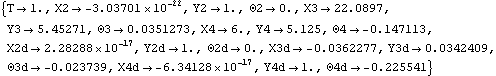
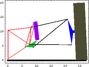
SolveMech is used to seek a solution to the model with the chassis 1.5 units off of the ground.

This generates a list of 12 solution sets, spaced evenly from T = 0.5 to T = 3.5.

Graphics

Mechanism Image

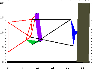
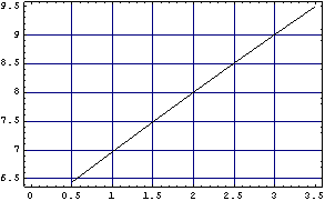
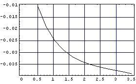
Animation

The following input will generate the series of 12 graphics in the animation cell at the beginning of this notebook.

Damper Length

Since the length of the damper is of primary importance to the operation of the suspension, an expression is created that represents the damper length as a symbolic function of the coordinates of each body.

Here is the damper length at T = 2.0.

Since the value of rodlength was set after SetConstraints was run, rodlength is still a variable in the equations generated by SetConstraints. Thus, it can be changed at any time.

Using the solution rules postab that were developed previously, damper length as a function of time is plotted with ListPlot.

Velocity Analysis

To analyze the velocity of the bodies in the model, components of the mathematical model must be differentiated with respect to time. This is done automatically when SolveMech is called with the Solution->Velocity option.

Note that the velocity solution is a superset of the position solution previously obtained.

Modeler2D contains a small set of velocity-based output functions, such as DDistanceDT, which returns the time derivative of Distance.

The same result is obtained by differentiating the expression returned by Distance with Dt.

A table of velocity solutions veltab is created in the same way that the table of location solutions postab was.

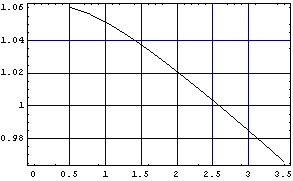
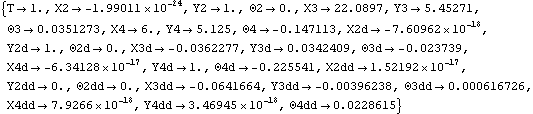
This plot shows that the velocity of the damper, relative to the velocity of the wheel, is increasing as the suspension of the car is compressed. Thus, the suspension is "rising rate" suspension.

Acceleration Analysis

To analyze the acceleration of the bodies in the model, components of the mathematical model must be differentiated twice with respect to time. This is done automatically when SolveMech is called with the Solution->Acceleration option.

Analogous to the velocity solution, the acceleration solution returned is a superset of the position and velocity solutions. Some acceleration output functions are available, such as D2DistanceDT2.

To avoid wasting computation time, SolveMech is able to update existing position (or position and velocity) rules without resolving for the lower-order solutions. The following example shows how SolveMech is passed an existing location solution (LastSolve[]) to be updated to a velocity solution. The CheckRules->False option prevents SolveMech from checking the validity of the solution rules that it is passed.

It took little time to update the current position solution with a velocity solution, while it takes longer to find both the position and velocity solutions.

This timesaving method is used to update the table of velocity rules veltab with the acceleration solution.

Here is a plot of the second derivative of the damper length with respect to time, T.

End