Spatial Follower

Example Mechanism for Modeler3D's Parametric Design Synthesis Functions

by Robert Beretta

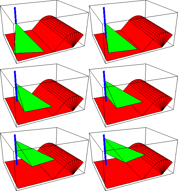
Spatial Follower Animation

Discussion

Follower Function

This notebook uses MechanicalSystems to analyze the motion of a spatial cam-follower mechanism. The motion of the follower is quite simple. The follower is fitted over a vertical post on the ground. The follower is free to slide up and down on the post, and to rotate. The rotation of the follower is enforced by a driver that pushes on the corner of the follower, in the horizontal plane. The remaining vertical degree of freedom of the follower is controlled by the contact between the tip of the follower and the ground--as the follower rotates, the tip first slides along the horizontal plane of the base plate, then it contacts and slides up the inclined plane, and finally the tip passes onto and over the cylindrical top surface of the follower.

Follower Model

The follower mechanism consists of two bodies.
1. Ground    (black)
2. Follower    (red)

Kinematic Model

Preparation

The Modeler3D package is loaded into Mathematica with the Needs command.

The following symbols are used to reference each of the bodies in the follower mechanism.

Body Definitions

Ground

Ten points are defined on the ground (body 1).
P1, P2, P3, and P4. The four corners of the bottom plate. The parameter a sets the X location of the intersection of the inclined plate and the bottom plate.
P5 and P6. The two ends of the line of intersection of the inclined plate and the cylinder.
P7 and P8. Two points on the axis of the cylinder. The parameter b sets the X location of the axis of the cylinder.
P9. The bottom of the pivot axis of the follower.
P10. The top of the pivot axis of the follower.
Two more parameters, x and z, are used locally just to simplify the coding.

Follower

Four points are defined on the follower (body 2).
P1. The point where the driver attaches to the follower, which is also the local origin.
P2. The point where the tip of the follower contacts the ground body.
P3. The bottom of the pivot axis of the follower.
P4. The top of the pivot axis of the follower.

Build bodies

The data contained in each of the body objects is entered into the current model with the SetBodies command.

Constraint Definitions

Four constraints, including one driving constraint, and one artificial constraint to add an extra variable c to the model are used to model the follower mechanism. First, c is cleared in case it currently has a value.

Constraints for the follower

1. Cylindrical4. A cylindrical joint between a vertical post on the ground and a vertical hole in the follower. This is a four degree of freedom constraint, the two remaining degrees of freedom being that the follower can rotate about its axis affixed to the ground, and it can slide up and down that axis.

2. RelativeX1. A driving constraint sets the X location of point 1 on the follower to be a function of T, and of other obscure dependent variables, just to be different.

3. TimeSwitch. A three-stage time switching constraint between the follower and the ground enforces that the tip (point 2) of the follower slide first along the base plate of the ground, then along the inclined plate, and finally over the top of the cylindrical upper surface. The switch times t1 and t2 are not known exactly at this time, so they will be determined later.

Additional constraint

4. Constraint. This one degree of freedom, user-defined constraint simply defines a variable c, adds it to the model's dependent variable list, and adds a constraint that sets c equal to zero.

Build constraints

The data contained in each of the constraint objects is incorporated into the current model with the Modeler3D SetConstraints command.

Running the Model

Take a guess at the values of the switch times, t1 and t2.

CheckSystem tests for certain modeling errors. A return value of True is OK.

SolveMech[t] runs the current model at time t and returns a list of rules containing the values of all of the dependent variables in the model.

Switch Times

The correct values of the switch times can now be found with FindSwitchTime. This finds switch time number 1 in constraint number 3.

SolveMech is called with the Solution->Velocity option just to get the current initial guess a little closer to what is known to be the correct location.

The TangentConstraint->True option must be used because there is no velocity discontinuity in the mechanism motion as it passes from the second to the third stage of the TimeSwitch.

Graphics

Follower Image

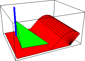
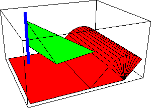
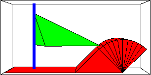
Animation

This creates a table of 15 position solutions, spaced evenly from T = 0 to 2, after resetting the initial guesses.

The following input generates a series of 16 graphics that can be animated.

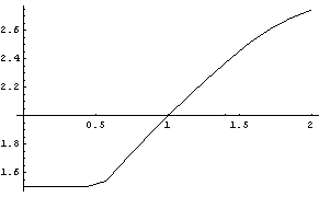
Position Plots

Here is a plot of the height of the follower.

Velocity

Here is the velocity of the top of the follower axis.

Acceleration

Here is the X acceleration of the local origin of the follower. The reason that this is nonzero is because the driving function in constraint 2 is a nonlinear function of other dependent variables that has a nonzero second derivative.

Coupled Systems

Location Couples

The following section illustrates the use of the SetCouple and SolveCouple functions. These functions are used here to adjust the values of parameters a and b (which were previously added to the model) so as to satisfy a specified mathematical condition, given as an equation with the head Equal.

Here is an expression that represents the Z location of the top of the follower.

Here is the value of the expression when T is equal to an arbitrary value T = 70.

The following SetCouple command effectively says "find the value of the parameter a, such that the equation is satisfied at time ." SetCouple returns a CoupleSystem data object that is solved with SolveCouple.

SolveCouple returns a list of rules, of the same form as those returned by SolveMech, including the new value of the parameter a.

Now that the parameter a has been set to its new value, the desired condition is satisfied.

The value of the single initial condition supplied to SetCouple (T) is changed with the InitialCondition option.

Note that these new values of the parameters have changed the mechanism geometry, such that the switch times found earlier are now invalid and must be updated.

Multitime Location Couples

SetCouple can solve for more than one variable, at more than one point in time.

The following SetCouple effectively says "Simultaneously find the values of a and b, such that the equation is satisfied at , using an initial guess of g1 (defined earlier) and that the equation is satisfied at , using the initial guess of g2." SetCouple now returns two complete solution rules, one corresponding to each point in time.

This finds a solution that satisfies the same set of conditions, at two new values of time.

Velocity Couples

SetCouple can handle conditions that depend on velocity variables.

Two expressions are defined, one the height of the top of the follower axis, and the other the vertical velocity of the follower axis.

The following SetCouple effectively says "Simultaneously find the values of a and b, such that the equations and are both satisfied at , using the current default initial guess LastSolve[]."

Multiconfiguration Velocity Couples

Coupled systems can be used to seek a solution that satisfies a location condition at one time and a velocity condition at another.

The following SetCouple seeks values for a and b that satisfy two constraints at two different configurations of the follower mechanism.

In this case, SolveCouple returns a list of two complete solution sets, one at and one at .

Free-Time Couples

Instead of solving only for parameters, SetCouple can use the time variable as one degree of freedom.

The option, Time->Free is used to tell SetCouple to consider the time variable to be a dependent variable.

Acceleration Couples

SetCouple can handle conditions that depend on acceleration variables.

FindTime

FindTime offers a subset of the functionality of SetCouple; it simply searches for the point in time at which an equality is satisfied.

Loaded Systems

Loads

A gravitational load is applied to the model with Gravity. This function applies the force to all of the bodies in the current model, which in this case is only one moving body.

SetLoads incorporates the force objects into Mech's internal database.

The following example gives the reaction force that constraint 2, the driving constraint, applies to the follower, calculated about point 1 on the follower. Reaction forces are returned in the format {{Fx, Fy, Fz}, {Mx, My, Mz}}.

Static FindTime

FindTime and SetCouple can handle conditions that are functions of constraint reaction forces.

Dynamic FindTime

The Solution->Dynamic option causes the accelerations to be calculated, and the inertia of the model to be included in the force analysis.

The Solution->Dynamic option must also be supplied to FindTime, or it would simply calculate the static solution, because nothing in the supplied condition implies that it must be dynamic.

Other Load Functions

Loads returns the sum of the external loads applied to a body, calculated about its origin.

The sum of all the loads applied to a body, in static mode, must equal zero.

Reaction can also return the effective load on a parameter.

Friction

A friction force is applied to the follower with a Force object. A friction force is simply a force whose magnitude is a function of another force. The Velocity term sets the direction of the force to be the opposite of the velocity of the point of contact.

The reaction at the driver is now much higher than it was with no friction.

Time Switching Forces

A TimeSwitch force turns on and off at specified points in time, analogous to the TimeSwitch constraint.

Here is the reaction at the driver just after the force has switched.

Here is the reaction at the driver just before the force has switched.

Static Equilibrium

In the following example, SetFree and SolveFree are used to find the equilibrium configuration of the model.

Three forces are defined: one that is a constant force, Gravity, one that is a function of location, Force, and one that is a function of velocity, Force. For an equilibrium location solution to exist, some of the forces must be functions of location. For an equilibrium velocity solution to exist, some of the forces must be functions of velocity. An equilibrium acceleration solution requires that masses be present, which effectively introduces some forces that are functions of acceleration.

SetFree seeks the equilibrium solution to the current model with specified constraints dropped to make the model underconstrained. By dropping constraint 4, the dependent variable c, which was held constant, becomes a variable.

Note that c has taken on a nonzero value.

Velocity Equilibrium

Zeroth-order initial conditions are required to find a velocity equilibrium solution.

To achieve velocity equilibrium at this initial condition, the parameter c must be changing at some nonzero rate.

If the initial condition is changed to the static equilibrium condition, the velocity equilibrium solution is at a dead stop. This is implied by the fact that the variable cd has a value of -1, which exactly cancels the first derivative of the time variable, 1.

Acceleration Equilibrium

Zeroth- and first-order initial conditions are required to find a velocity equilibrium solution.

The acceleration equilibrium solution requires that the parameter, c, have a nonzero acceleration.

If an acceleration equilibrium solution is found with the velocity equilibrium solution used as an initial condition, the second derivative of the parameter c is not zero because the inertia forces on the model are dependent on angular velocity. These forces were not included in the velocity equilibrium solution, so some acceleration must be present to account for them.

However, if the static equilibrium configuration is used as the initial condition, all of the angular velocities are zero so the second derivative of the parameter c is zero.

End