8.3.3 Friction ExampleTo demonstrate the application of Coulombic friction to a Mech mechanism model, a 2D model of a slider on an inclined ramp is developed. The model consists of one moving body, the slider.
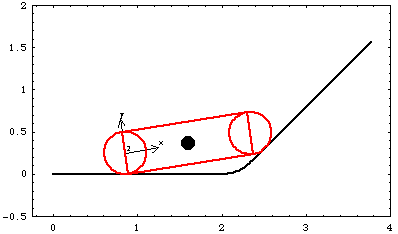
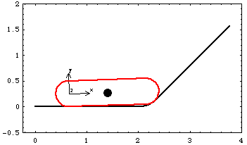
As the slider is pushed along its track on the ground body, it travels along the initial horizontal part of the track until the tip of the slider encounters the upward turn of the track. The tip then progresses up the inclined ramp while the heel of the slider stays on the horizontal section. Coulombic friction is modeled at the two sliding interfaces at the tip and the heel of the slider. The Modeler2D TimeSwitch function is used to switch between the different friction forces as the tip of the slider passes from one section of the ramp to the next. This loads the Modeler2D package. Here is a graphic of the 2D slider-ramp model.

BodiesTwo body objects are defined for the slider-ramp model. The ramp (body 1) requires five point definitions.
P1 is the origin of the ramp.
P2 is a point directly to the right of the origin to define the lower flat of the ramp.
P3 is the center point of the curved section of the ramp.
P4 and P5 are two points that define the upper flat of the ramp.The slider (body 2) requires two local point definitions.
P1 is the center of the heel of the slider, which is the local origin.
P2 is the center of the tip of the slider.Note that points 3, 4, and 5 on the ramp are defined as functions of two user-defined variables radius and incline, so that the radius at the curve of the ramp and the angle of the incline can be changed easily.
Because a gravitational force will be applied to the slider, the mass and centroid location are defined in the slider's body object. Names are defined for each of the bodies in the model. Here are the body objects for the slider-ramp. The body properties are added to the current model. ConstraintsThree constraints, one of which is a driving constraint, are required to model the slider-ramp mechanism. A RelativeX1 constraint controls the horizontal position of the heel of the slider. This constraint is a driving constraint because it is functionally dependent on the time variable T.A RelativeY1 constraint keeps the heel of the slider in contact with the ramp.A TimeSwitch constraint keeps the tip of the slider in contact with the ramp. The TimeSwitch constraint has three stages:
1. A PointOnLine1 constraint keeps the tip of the slider in contact with the horizontal section of the ramp.
2. A RelativeDistance1 constraint keeps the tip of the slider in contact with the curved section of the ramp.
3. A PointOnLine1 constraint keeps the tip of the slider in contact with the inclined section of the ramp.The value of the initial switch time determined by inspection is 0.5. However, the value of the second switch time is more difficult to determine analytically, so it is left as the symbol swtime and the FindSwitchTime function is used to find a numeric value. Here are the constraint objects for the slider-ramp model. Here, the constraints are added to the current model. RuntimeBefore the model can be run the undefined symbols, incline, radius, and swtime, must be defined. $MechVariables returns the names of any symbols that have been recognized as being part of the current model. Here is a Mech utility.
Out[52]= |  |
The embedded symbols are explicitly defined. Now the model is run at T = 0.65.
Out[56]= |  |
Here is the slider-ramp model at T = 0.65.

Switch TimeNow the exact value of swtime can be found with FindSwitchTime. Because the slider passes tangentially from the curved section of the ramp onto the inclined section (which implies that there is no discontinuity in the velocity of the slider at the transition), the TangentConstraint option must be used with FindSwitchTime. This option tells FindSwitchTime to look for the point of velocity equality instead of just location equality. Find switch time 2 in constraint 3.
Out[57]= |  |
LoadsThe goal of this example is to determine the force required to push the slider around the curved section of the ramp and up the incline, with gravity pulling down on the slider, and friction between the slider and the ramp at both ends.
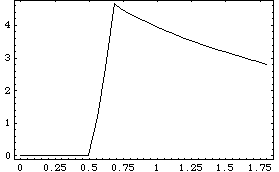
First, gravity is applied without any friction forces. A plot of the force required to push the slider is made from a list of solutions returned by SolveMech. Here is a gravitational load. The model is run from T = 0.0 to 1.8.
Out[59]= |  |
Here is a plot of the driving force.

Out[60]= |  |
Now a friction force is added to the left end of the slider. This is fairly straightforward, as the line of action of the force is constant throughout the motion of the slider. The force is applied to the slider and the line of action is along the surface of the ramp. The magnitude of the force is equal to the coefficient of friction times the normal force at the left end of the slider, which is the Y reaction to constraint 2. Here is the left end friction load. The symbol cf is the coefficient of friction. Now a friction force is added to the right end of the slider. This is rather complicated, as the line of action of the friction force changes as the slider passes from one section of the ramp to another.
The friction force is applied to the slider, but the line of action is along the surface of the ramp. On the two flat sections of the ramp, the friction force is applied in the same manner as the force on the left end of the slider. However, the line of action of the force around the curve on the ramp has to be developed directly with vector algebra.
Although the line of action changes as the slider moves through the different stages of the ramp, the magnitude of the normal force is always equal to the coefficient of friction times the magnitude of the reaction force of constraint 3, even though constraint 3 is changing from one constraint type to another.
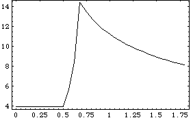
TimeSwitch is used to switch between the forces in exactly the same manner as it is used to switch constraints, without the constraint number argument. Since the forcing functions switch at the same times as the constraints, the same switch times can be used. Here is the right end friction load All of the defined loads are added here to the current model. SolveMech is called with intermediate times in between the beginning and end times that are explicitly included in the points in time that are solved for. This ensures that a data point is included exactly at the peak of the force plot. The model is now run through a range of 30 points in time, including the two switch times.
Out[66]= |  |
Here is a plot of the driving force.

Out[67]= |  |
|