|
9. Parametric Design OverviewThis chapter covers the use of MechanicalSystems' parametric design synthesis functions, SetCouple and SolveCouple. These functions allow the user to specify one or more geometric conditions that are to be satisfied, along with the names of parameters that are to be varied in an attempt to satisfy them. Coupled systems can be used to satisfy several geometric conditions that are specified at different configurations of the model, or conditions that are dependent on velocity, acceleration, or constraint reactions.
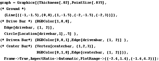
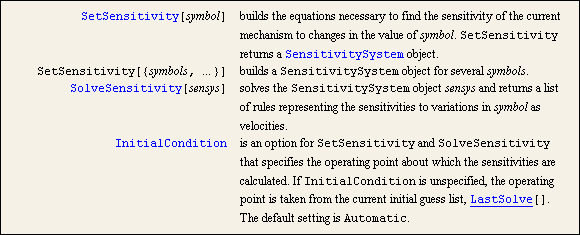
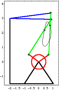
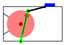
The SetSensitivity and SolveSensitivity functions find the linearized sensitivity of all of the dependent variables in a model to variations in specified parameters. These functions are used to perform a linearized tolerance analysis on a multibody system. 9.1 Coupled ModelsThe simplest invocation of the SetCouple and SolveCouple functions is to allow a model parameter or parameters to be varied in an attempt to satisfy some geometric condition at one point in time. In this section a planar model of a four-bar mechanism is developed, and the lengths of the links in the four-bar mechanism are adjusted to achieve various desired geometric design goals. 9.1.1 2D Example MechanismThis subsection develops a planar model of a classic four-bar mechanism. The driving input to the model is to specify the rotation of bar 2, the drive bar. Because the drive bar is the shortest link in the model, the driven bar and center bar simply oscillate as the drive bar progresses through each full turn. Driven in this manner the model has no singular configurations. This loads the Modeler2D package. Here is a graphic of the four-bar model.
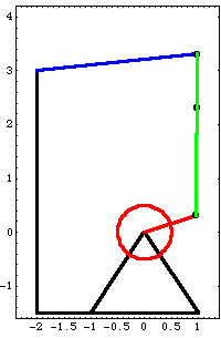
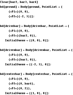
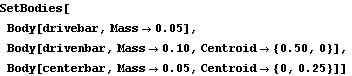
BodiesFour body objects are defined for the four-bar mechanism model. Each body in the model is simply a two-ended bar, so only two local points are defined on each body. Each body is attached to one neighboring body at its local origin and another neighboring body at an offset point on the local x or y axis. Body 4, the center bar, has a third point defined that is used only as a point of reference to measure the motion of the model.
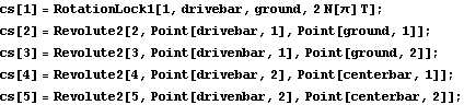
The body objects are defined such that the length of each bar is a symbolic parameter that can be changed at a later time. Names are defined for each of the body numbers in the model. Here are the four body objects for the four-bar model. The body objects are incorporated into the current model with SetBodies. ConstraintsFive constraints, one of which is a driving constraint with explicit dependence on time, are used to model the four-bar mechanism. A RotationLock1 constraint controls the rotation of the drive bar as a function of T. Four Revolute2 constraints model the revolute joints at each end of the four bars. Here are the five constraint objects for the four-bar model. The constraint objects are incorporated into the current model with SetConstraints. RuntimeBefore the model can be run, the symbols bar2, bar3, and bar4 that determine the length of the each bar must be defined. The SetParameters function is used to make the symbols formal parameters so that they are recognized by SetCouple. The symbolic lengths of each bar are defined.
Out[20]= |  |
Now the model is run at T = 0.05.
Out[21]= |  |
Here is a plot of the four-bar mechanism with the locus of a point on the center bar.
9.1.2 Solving for One ParameterThe coupled system building and solving functions. Mech's SetCouple and SolveCouple functions are now used to adjust the length of the drive bar bar2. In the four-bar's current configuration, the X coordinate of point 3 on the center bar is 0.898 at T = 0.1. The following example uses a coupled system to find the length of the drive bar that causes the X coordinate of point 3 to be equal to 0.8 at T = 0.1. Here is the current X coordinate of point 3 on the center bar.
Out[23]= |  |
SetCouple basically adds a degree of freedom to the mechanism model by allowing a parameter to become a dependent variable, and also adds an equation to constrain the new degree of freedom. The following command essentially says "adjust the value of bar2 such that the X coordinate of point 3 on the center bar is equal to 0.8 at the current default time T = 0.1."
The current default initial guesses obtained from LastSolve[] are used as the initial guesses for the CoupleSystem, unless otherwise specified. The current value of the parameter bar2 is used for its initial guess. This builds the CoupleSystem object.
Out[24]= |  |
SetCouple returns a CoupleSystem object that is solved with SolveCouple. The CoupleSystem object contains a new set of constraint equations that include all of the constraints in the current model, plus one. The list of rules returned by SolveCouple is of the same form as the rules returned by SolveMech. This solves the CoupleSystem object and finds a new value of bar2.
Out[25]= |  |
The new value of the parameters bar2 is added to the current parameters list.
Out[26]= |  |
This shows that the desired condition is satisfied.
Out[27]= |  |
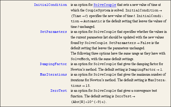
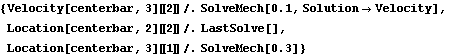
Options for SolveCouple. Without building a new CoupleSystem object, cpsys can be re-solved at a new value of time by using the InitialCondition option. Note that the InitialCondition option expects a setting of the form Time -> t, not T -> t. The CoupleSystem is solved again with a new value of time.
Out[28]= |  |
The contents of the current parameters list are updated.
Out[29]= |  |
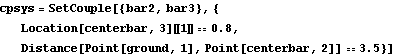
9.1.3 Solving for Multiple ParametersBuilding coupled systems with multiple parameters. Multiple parameter values are solved for by supplying an equal number of geometric conditions to be satisfied. A coupled system is used here to find the values of bar2 and bar3 that simultaneously cause the X coordinate of point 3 on the center bar to be 0.8 and the distance from the global origin to point 2 on the center bar to be 3.5, both at T = 0.1. This finds the X coordinate of point 3 and the distance from the origin to point 2 at T = 0.1.
Out[30]= |  |
This builds the CoupleSystem object.
Out[31]= |  |
This solves the CoupleSystem object and finds new values for bar2 and bar3.
Out[32]= |  |
This shows that the desired conditions have been satisfied.
Out[33]= |  |
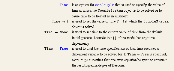
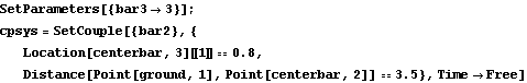
In all the preceding examples, the value of time T at which the coupled model has been solved has been taken from the default initial guess list. The Time option is used to explicitly set the value of time in the CoupleSystem object, or to specify that time is a dependent variable. An option for SetCouple. Instead of fixing time at 0.1, time can be a dependent variable to be solved for. The following example seeks the values of bar2 and T that satisfy the same pair of conditions that were used in the previous example. The parameter bar3 is reset to its original value before building the new CoupleSystem.
Out[35]= |  |
Here is the solution for T and bar2.
Out[36]= |  |
The desired conditions are satisfied.
Out[37]= |  |
Undocumented Graphics Generation9.2 Multiple Configuration CouplesThe SetCouple and SolveCouple functions can be used to find the values of several parameters that simultaneously satisfy several geometric conditions at different configurations of the model, at different points in time. 9.2.1 Solving for Two ParametersBuilding coupled systems across multiple configurations. The InitialGuess and Time options are used somewhat differently than standard Mathematica option usage because one specification for time and one set of initial guesses must be given for each separate mechanism configuration. The Time option must be specified for a multiple configuration CoupleSystem because the default setting sets the value of time to be the same for all configurations, making all configurations identical. Since the Compiled option applies to the entire CoupleSystem, it can appear in any part of the SetCouple command.
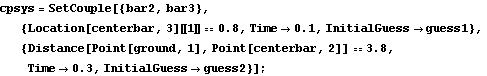
The following example uses the four-bar model that was developed in Section 9.1. A coupled system is used to adjust the lengths of both the drive and driven bars so as to meet two geometric conditions that are satisfied at two different points in time. The X coordinate of point 3 on the center bar is set to 0.8 at T = 0.1, and the distance from the global origin to point 2 on the center bar is set to 3.8 at T = 0.3.
Because the coupled system is simultaneously solved in two different mechanism configurations, the same initial guess for both configurations may not be acceptable. Therefore, the InitialGuess option is used to explicitly specify initial guesses for each configuration. Here are two initial guesses for the two configurations. Here are parts of the two conditions at the two initial configurations.
Out[41]= |  |
This builds the CoupleSystem object. A CoupleSystem object that spans multiple configurations has a unique solution at each configuration. Thus, SolveCouple returns a nested list of solution rules with each list corresponding to one configuration of the mechanism. This solves the CoupleSystem object and finds new values for bar2 and bar3.
Out[43]= | 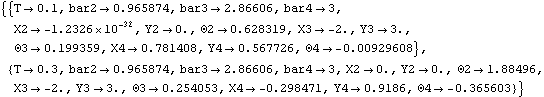 |
This shows that the desired condition is satisfied.
Out[44]= |  |
9.2.2 Solving for Multiple ParametersIt is possible to specify any number of geometric conditions to be satisfied at any number of different mechanism configurations, however, it is certainly not possible to satisfy any arbitrary set of conditions. A CoupleSystem object built by SetCouple may have no solution, or it may have stiff singularities at points very close to a valid solution, making it difficult to converge the model. The following example demonstrates a useful technique for slowly coaxing a model towards a desired solution with SolveCouple.
In the following example, a coupled system is used to find the values of bar2, bar3, bar4, and T that satisfy four different geometric conditions at two different points in time. The X and Y coordinates of point 3 on the center bar are specified at T = 0.1, and the X and Y coordinates of point 3 on the center bar are specified at an arbitrary time T > 0.1, effectively specifying that point 3 on the center bar must pass through a given point in the global reference frame. Here is the current location of point 3 at T = 0.1 and T = 0.3.
Out[46]= |  |
Out[47]= |  |
First, a CoupleSystem object is built that has very unambitious goals. This system simply tries to satisfy a set of conditions that are already approximately satisfied. Then, the coordinate goals k1, k2, k3, and k4 are changed, slowly pulling the solution of the model away from its original configuration. The new parameters, k1 to k4, are added to the parameters list. Note that the parameters bar2, bar3, and bar4 are approximately equal to their original values.
Out[50]= |  |
When SolveCouple is called with a symbol that evaluates to a CoupleSystem object as its first argument, SolveCouple updates the initial guesses contained within the CoupleSystem object to the new values found to be the solution. Therefore, independent parameters can be slightly tweaked between successive runs of SolveCouple, with each run nudging the model slightly closer to the desired solution. The parameters are repeatedly changed and the model is re-solved.
Out[52]= |  |
Out[54]= |  |
Out[56]= |  |
Out[58]= |  |
Here is the four-bar mechanism at T = 0.1 and T = 0.396, with the locus of point 3 on the center bar.
The k1-k4 parameters are removed from the parameters list. 9.3 Velocity and Acceleration CouplesCoupled systems are not limited to geometric conditions that involve only mechanism body location and orientation. Velocity and acceleration terms may be included in the conditions to be satisfied. However, the parameters that are varied in attempting to satisfy the conditions are assumed to be constant. Mech parameters never have nonzero derivatives. 9.3.1 Solving for Two ParametersTo demonstrate the use of coupled systems to satisfy higher-order conditions, the four-bar model developed in Section 9.1 is used again. In the following example, the lengths of the drive bar and the driven bar are adjusted to satisfy two geometric conditions that are specified in two different mechanism configurations. One of the conditions is a first-order expression, specifying a component of the velocity of a point.
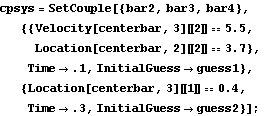
In the following example, bar2 and bar3 are adjusted so that the X coordinate of point 3 on the center bar is 0.4 at T = 0.3, and the Y velocity of point 3 on the center bar is 6.0 at T = 0.1. Initial guesses are specified for each configuration, and the initial guess for configuration 1, which contains the velocity condition, includes velocity terms. Here are two initial guesses for the two configurations. This builds the CoupleSystem object. This solves the CoupleSystem object.
Out[65]= |  |
The nested list of rules returned by SolveCouple has one complete solution for each of the two mechanism configurations. Note that SolveCouple automatically determined that a velocity solution was needed for the first configuration by the presence of first-order terms in the geometric condition. This shows that the desired goal has been achieved.
Out[66]= |  |
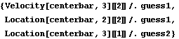
9.3.2 Solving for Multiple ParametersThis last example of the use of coupled systems with velocity dependence uses two geometric conditions that are satisfied in one configuration, and one condition that is satisfied in another configuration. One of the conditions is an expression involving velocity.
bar2, bar3, and bar4 are adjusted so that the X coordinate of point 3 on the center bar is 0.4 at T = 0.3, the Y velocity of point 3 is 5.5, at T = 0.1, and the Y coordinate of point 2 on the center bar is 3.7, also at T = 0.1. Here are the current values of the coordinates that are to be specified.
Out[67]= |  |
This builds the CoupleSystem object. This solves the CoupleSystem object.
Out[69]= |  |
This shows that the conditions are now satisfied.
Out[70]= | 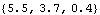 |
9.4 Load-Dependent CouplesCoupled systems may be built with mathematical conditions that depend on reaction forces in the mechanism, instead of geometric conditions that depend on body locations and velocities. Such expressions contain the Lagrange multiplier terms ( 1, 2, ...) that are used to resolve static and dynamic reaction forces in a model. The four-bar mechanism is used to demonstrate this, after adding applied forces and gravity to the model so that the joint reactions are nonzero. 1, 2, ...) that are used to resolve static and dynamic reaction forces in a model. The four-bar mechanism is used to demonstrate this, after adding applied forces and gravity to the model so that the joint reactions are nonzero. 9.4.1 Loads on the Four-Bar ModelThe four-bar mechanism defined in Section 9.1 now has a constant moment applied to the driven bar and gravitational force applied to all bodies. This sets nonzero masses for each body. Here is a clockwise moment applied to the driven bar, and gravity applied to all bodies. 9.4.2 Solving for a ParameterA coupled system is used to find the length of the drive bar that causes the reaction moment at the driving constraint to be equal to 0.5. The driving constraint, number 1, is a RotationLock1 constraint constraining the rotation of the drive bar. Since this constraint only controls the rotation of the drive bar it can support no forces, only a moment. Thus, the reaction force at the constraint is exactly zero. Here is the reaction force and moment that the driving constraint applies to the drive arm.
Out[74]= |  |
At T = 0.2, the driving constraint must apply a 0.65 unit moment to the drive bar to counteract the gravitational forces and the moment applied to the driven bar. A CoupleSystem object is built that seeks the value of bar2 that results in a reaction moment of 0.5 units at T = 0.2. This builds the CoupleSystem object.
Out[75]= |  |
This solves the CoupleSystem object.
Out[76]= |  |
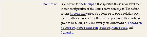
As with the examples given in Section 9.2, coupled systems can be built that couple multiple mechanism configurations. The conditions to be satisfied in such a system can be a mix of geometric conditions and algebraic conditions based on reaction forces. 9.4.3 Dynamic SolutionsAn option for SetCouple. In all of the preceding examples, SetCouple has been called with the default setting for the Solution option, Solution -> Automatic. SetCouple automatically upgrades the Solution setting to Velocity when first-order terms are encountered in the equations, or to Acceleration when second-order terms are encountered. SetCouple chooses the Static setting if Lagrange multipliers are encountered due to reaction forces in the equations.
However, SetCouple does not automatically choose the Kinematic or Dynamic settings for Solution unless first- or second-order terms and Lagrange multiplier terms appear in the equations, even though a dynamic solution (that includes inertial forces) may be desired. In the following example a CoupleSystem object is built with exactly the same inputs as in the previous example, but the Solution -> Dynamic option causes inertial forces to be included, resulting in a different solution. Here is the reaction that the driving constraint applies to the drive arm, including dynamic forces.
Out[78]= |  |
With dynamic forces included, the reaction moment at the drive bar is reduced to only 0.48 units at T = 0.2. A new CoupleSystem object is built that seeks the value of bar2 that results in a reaction moment of 0.5 units at T = 0.2, the same reaction moment that was sought in the previous example. This builds the CoupleSystem object with a dynamic formulation.
Out[79]= |  |
Note that the resulting length of the drive bar is quite different than was calculated using only static forces. This solves the CoupleSystem object.
Out[80]= |  |
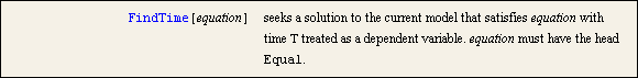
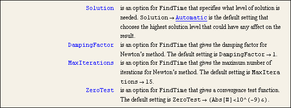
9.4.4 Dependent TimeA combined form of SetCouple and SolveCouple. FindTime options. FindTime is essentially a special combined form of the SetCouple and SolveCouple functions that accepts only one condition to be satisfied, and considers time to be the only new dependent variable. This seeks the time at which the reaction on the drive bar is equal to 8.
Out[81]= | 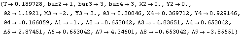 |
FindTime automatically pulls its initial guesses from the current default initial guess list LastSolve[] and it updates the initial guess list with the new solution that it finds. This shows that the specified condition has been met.
Out[82]= |  |
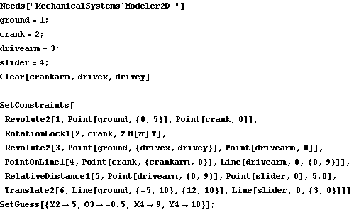
This clears the parameters list. 9.5 SensitivityMechanicalSystems' sensitivity analysis functions are used to perform linearized tolerance analysis on multibody mechanisms. Similar to the SetCouple and SolveCouple functions discussed in the previous sections, SetSensitivity and SolveSensitivity are used as a pair to build and solve SensitivitySystem objects. A planar example mechanism is developed in this section that is used to demonstrate the use of these functions. 9.5.1 Example MechanismThe quick-return mechanism model that was developed in Section 3.1 is used here to demonstrate the use of sensitivity systems. The model is redefined as follows in abbreviated form. Here is the entire quick-return model. Note that three parameters were added to the model that are used in the following sensitivity analysis: crankarm, which is the local x coordinate of the crankpin on the crank, drivex and drivey, which are the X and Y coordinates of the attachment point of the drive arm to the ground, respectively. Here is a graphic of the quick-return mechanism.
9.5.2 Sensitivity to Parameter VariationsThe quick-return model contains three undefined parameters: crankarm, drivex, and drivey. We wish to find the sensitivity of the location of each body in the mechanism to small changes in these parameters, about some operating point. The sensitivities are not constant, they change as the mechanism moves through a complete cycle. Thus, the maximum sensitivity at any point in a cycle is of interest. The values of the parameters are set and the body locations are found at the initial operating point.
Out[10]= |  |
The sensitivity functions. First, the sensitivity to variations in the crankarm parameter are found. This builds the SensitivitySystem object.
Out[11]= |  |
This solves the SensitivitySystem object.
Out[12]= |  |
The solution returned by SolveSensitivity is identical in form to the solution returned by SolveMech[time, Solution -> Velocity]. The difference is that the velocity terms X2d,  3d, and so on, do not represent dX2/dT and d3/dT; they represent dX2/dcrankarm and d3/dcrankarm. Because the results from SolveSensitivity are returned in this form, it is possible to use any of the MechanicalSystems' output functions, differentiated once, to find the sensitivity of more complicated quantities to changes in the parameter. 3d, and so on, do not represent dX2/dT and d3/dT; they represent dX2/dcrankarm and d3/dcrankarm. Because the results from SolveSensitivity are returned in this form, it is possible to use any of the MechanicalSystems' output functions, differentiated once, to find the sensitivity of more complicated quantities to changes in the parameter. Here is the sensitivity of the distance from the crank center to the slider origin to changes in crankarm.
Out[13]= |  |
Out[14]= |  |
9.5.3 Multiple ParametersIf multiple symbols are passed to SetSensitivity, SolveSensitivity returns a nested list of solutions, one for each symbol. Here a SensitivitySystem object is built and solved with three parameters. Here is the sensitivity of the slider location to variations in each of the parameters.
Out[17]= |  |
To plot the sensitivity of the slider location to changes in these three parameters, a set of solutions at several operating points is generated and used as initial conditions for SolveSensitivity. This resets the initial guesses and seeks 25 solution points through a full turn of the crank. Now SolveSensitivity is applied with each of the position solutions serving as an initial condition. Here is a plot of the sensitivities.
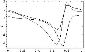
Out[21]= |  |
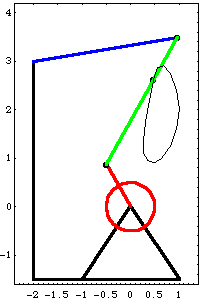
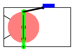
Note that the sensitivities are rather large near 3/4 turn of the crank. This is to be expected with a quick-return mechanism because of the high leverage ratio between the crank and the slider during the return stoke. The largest negative sensitivity is the sensitivity to the X coordinate of the drive arm rotational axis drivex, when the crank is at 3/4 turn. Here is the quick-return mechanism at 3/4 turn of the crank.
|