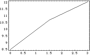
4.2.6 InterpolationMechanicalSystems provides a function that enhances the functionality of the Mathematica Interpolation function when used with a Mech model. This function is described in Section 3.2, but this subsection covers its capability of automatically utilizing higher-order data to obtain higher accuracy the interpolated results. Interpolation utilities. To demonstrate the use of TimeInterpolate, we must have an expression to interpolate and a list of rules to interpolate it over. shocklength is the length of the damper in the pull-rod suspension model. Here is a list of three location solutions. The following plot shows a course representation of the shock length versus time. Only three data points were calculated by the previous call to SolveMech, T = 3, 1.5, and 0, so the ListPlot graphic consists of only two straight line segments. Here is a plot of the shock length versus time.
Out[61]= |  |
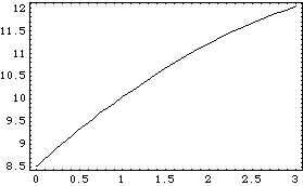
If we use TimeInterpolate to interpolate among the three points, the curve looks much smoother, but it is still a very poor representation, because there is no way for the InterpolatingFunction to know that the curvature increases as T approaches zero. Here we interpolate the shock length function with a default InterpolationOrder that is too high.

Out[62]= |  |
Here is a plot of the zeroth-order representation of shocklength.
Out[63]= |  |
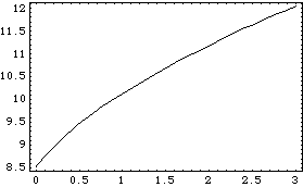
A new table of three solution rules is calculated, but this time velocity and acceleration data is included. To avoid recalculating all of the location solution points, SolveMech is passed the list of location solutions that have already been generated. This generates a new list of solution rules using the existing rules as initial guesses. The higher-order slope and curvature information contained in acctab is automatically included in the new InterpolatingFunction object returned by TimeInterpolate. Again, we interpolate the shocklength function. Here is a plot of the second-order representation of shocklength.
Out[66]= |  |
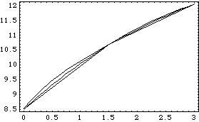
Here are the three plots shown together.
Out[67]= |  |
Interpolating SolutionsAnother method of applying interpolation is to directly interpolate the rules returned by SolveMech. SolveMech accepts the symbol Interpolation as an option name to tell SolveMech to interpolate the rules it returns. Note that SolveMech does not interpolate variables that are constant. An option for SolveMech. Because the Solution -> Acceleration option is given in the following example, the InterpolatingFunction objects returned contain slope and curvature information from the velocity and acceleration solutions. Here is a set of interpolated solution rules.
Out[69]= | 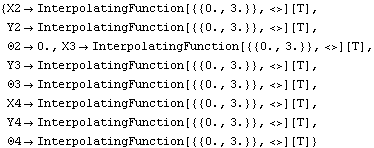 |
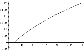
Here is another plot of shocklength.
Out[70]= |  |
|