4.2 Velocity and Acceleration OutputNow that the velocity and acceleration of each mechanism body has been calculated, useful output may be generated by developing expressions that are functions of Mech velocity and acceleration variables, and subjecting those expressions to the standard solution rules produced by SolveMech. 4.2.1 3D Example MechanismThe 3D MacPherson strut suspension model is used to demonstrate various methods of producing velocity and acceleration output with Mech. The model is redefined as follows in abbreviated form. The complete MacPherson strut suspension model follows. Here the model is run at T = 2.5 to prove that it still works.
Out[5]= |  |
4.2.2 Output FunctionsWhile Mech provides a wide array of output functions that return various quantities related to body location or orientation, only a small subset of those output functions are available in versions that are related to body velocities or accelerations. The most basic of those are the two higher-order analogies of the Location function. For each of the following functions, the point argument can be a Mech point object or just the arguments to a Mech point object. Velocity and acceleration output functions. The velocity of the steering tie rod attachment point on the wheel carrier is very near zero in the global reference frame because the chassis is allowed to move up and down while the bottom of the tire (the carrier body) remains in contact with the ground. Thus the motion of the carrier with respect to the ground is just a small tipping about the bottom of the tire. This calculates the velocity of a point.
Out[6]= |  |
A related velocity function. The velocity of the steering tie rod attachment point with respect to the chassis has a much larger vertical component, while the longitudinal and transverse components remain the same. The velocity of a point, relative to another body, is shown here.
Out[7]= |  |
Two functions provide the higher-order analogies to the Rotation function. 2D2D angular velocity and acceleration functions. 3D3D angular velocity and acceleration functions. Note that all Mech output functions formulate expressions in terms of derivatives of Euler parameters, or global angular velocities and accelerations, or local angular velocities and accelerations. Which form is returned depends on the settings of the Method and Coordinates options for SetSymbols that were in effect the last time that the model was built.
For example, the current model was built with the default Method -> Euler setting in SetSymbols; therefore, all output functions will return expressions in terms of derivatives of Euler parameters that can be replaced by a solution rule. Here is the angular velocity of the wheel carrier.
Out[8]= |  |
Out[9]= |  |
The Method -> Angular option is now used with SetSymbols. This changes the formulation of the Modeler3D output functions, but the numbers remain the same. The model is rebuilt with the Angular option setting. The angular velocity of the wheel carrier is the same.
Out[12]= |  |
Out[13]= |  |
Again, the internal representation of the angular velocity can be changed to local coordinates, but the numerical results from the output functions remain the same. The model is rebuilt again with local angular velocity representation. The angular velocity of the wheel carrier is still the same.
Out[16]= |  |
Out[17]= |  |
The only other output functions that are defined by Mech are the higher-order analogies to the Distance function. These two functions are defined largely for academic reasons, because they can be reproduced simply by differentiating the Distance function, as is shown in Section 4.2.3. Two more higher-order output functions. There is a slight difference between using the velocity output functions Velocity, DDistanceDT, and so on, and simply differentiating their first-order counterparts Location and Distance. The first- and second-order output functions use the Mathematica D operator to differentiate the local coordinates of each point, thereby assuming that the local coordinates are constant unless they are explicitly functions of time T. Here are the length, and the first and second derivatives of the length of the strut.
Out[18]= |  |
4.2.3 Differentiating ExpressionsAlthough Mech provides only a small number of predefined output functions that relate to velocity and acceleration, any expression that is written in terms of Mech dependent variables can be differentiated with Dt because definitions have been automatically made for Dt[X, T], where X is any Mech dependent variable. Now the model is rebuilt with the Method -> Euler setting. Here is the rate of change of the camber angle.
Out[21]= |  |
Out[22]= |  |
This generates a numerical result at T = 2.5.
Out[23]= |  |
Note that Dt automatically replaced derivatives of dependent variables with the appropriate symbols. This form of differentiation is valid even when crossing from Euler to angular coordinates.
Consider the following example. With the Method -> Euler setting for SetSymbols, differentiating the seven Modeler3D location coordinates associated with body 3 with respect to T has the apparent effect of appending a d to the name of each variable. These new symbols are explicitly included in the solution rules returned by SolveMech.
However, with the Method -> Angular option set, differentiating the seven Modeler3D symbols with respect to T produces different symbolic results. This shows the functional relationship between the Euler parameters and the angular velocity. After replacement with a SolveMech solution rule, the results are numerically identical. This shows the derivatives of dependent variables.
Out[24]= |  |
Out[25]= |  |
Out[26]= |  |
Now the model is rebuilt with the Method -> Angular option. The derivatives of dependent variables have changed form, but their values remain the same.
Out[29]= |  |
Out[30]= |  |
Out[31]= |  |
The same holds true for the local coordinate formulation.
Out[34]= |  |
Out[35]= |  |
Out[36]= |  |
Note that the only difference between the derivatives of the Euler parameters in terms of global or local coordinates is that a few of the signs are swapped. 4.2.4 Euler's AnglesAs shown in Sections 4.2.2 and 4.2.3, Euler parameters and their derivatives are directly related to the angular velocity vector of a spatial body, and a direct conversion between angular velocity and the derivatives of Euler parameters is possible. However, there is no vector representation of spatial angular orientation so other representations must be used.
One method of representing the angular orientation of a spatial body is to define a sequence of three finite rotations about three fixed axes that take a body from one orientation to another. These three rotations are called Euler's angles. Angular orientations represented by Euler's angles are readily converted to and from Euler parameters with a combination of Modeler3D output functions. Mech does not provide a single function to make this conversion, because there are many possible combinations of successive rotations that can be used to represent the angular orientation of a body.
The following example shows the general procedure required to convert an angular orientation from a sequence of finite rotations to a set of Euler parameters. In this particular case, the sequence of rotations are the most commonly used Euler's angles. Rotation 1 is a rotation phi about the global Z axis.Rotation 2 is a rotation theta about the X axis in the new reference frame created by rotation 1.Rotation 3 is a rotation psi about the Z axis in the new reference frame created by rotation 2.Here are the three rotation angles, and vector constants for each axis. A single rotation matrix that combines the three successive rotations is created by multiplying the rotation matrices associated with each. Out[43]//MatrixForm=
 |
The EulerParameters function is used to convert the rotation matrix to a set of Euler parameters.
Out[44]= |  |
The conversion of Euler parameters to a sequence of finite rotations is not such a straightforward process. The general procedure is to measure the angle between an appropriate pair of axes located in the global and local reference frames. The following example shows how to convert the Euler parameters eulpars back to three Euler's angles. Since Mech output functions that return expressions in terms of the symbolic Euler parameters are used, a list of replacement rules is needed.
Out[45]= |  |
Here is the second Euler's angle theta. It is the included angle between the two Z axes in the global and local reference frames.
Out[46]= |  |
Out[47]= |  |
Here is the first Euler's angle phi. It is the angle between the local Z axis and the global -Y axis, as viewed looking down onto the global X-Y plane.
Out[48]= |  |
Out[49]= |  |
Here is the last Euler's angle psi. It is the angle between the local Y axis and the global Z axis, as viewed looking down onto the local X-Y plane.
Out[50]= |  |
Out[51]= |  |
Any angular orientation can be represented by a single finite rotation about a fixed axis. This single rotation angle and axis are directly related to the Euler parameters so a direct conversion can be made with the Rotation function. Here is the single rotation about a fixed axis that is equivalent to the three successive rotations phi, theta, and psi.
Out[52]= |  |
Some readers may be more familiar with the use of quaternions to represent the orientations of spatial bodies. Quaternions are four-dimensional complex quantities, with associated rules for multiplication, that allow them to be used much like 3D rotation matrices. The numerical values of the four elements of the quaternion qw + qx i + qy j + qz k are equivalent to the numerical values of the four Euler parameters {eo, ei, ej, ek} representing the same orientation. Quaternions and Euler parameters are notationally and conceptually quite different, but they are computationally equivalent. 4.2.5 2D Example MechanismThe 2D pull-rod suspension model that was presented in Section 4.1 is used to demonstrate various methods of producing velocity and acceleration output with Mech. The model is redefined as follows in abbreviated form. Here is the complete pull-rod suspension model. Here the model is run at T = 2.5 to prove that it still works.
Out[58]= |  |
4.2.6 InterpolationMechanicalSystems provides a function that enhances the functionality of the Mathematica Interpolation function when used with a Mech model. This function is described in Section 3.2, but this subsection covers its capability of automatically utilizing higher-order data to obtain higher accuracy the interpolated results. Interpolation utilities. To demonstrate the use of TimeInterpolate, we must have an expression to interpolate and a list of rules to interpolate it over. shocklength is the length of the damper in the pull-rod suspension model. Here is a list of three location solutions. The following plot shows a course representation of the shock length versus time. Only three data points were calculated by the previous call to SolveMech, T = 3, 1.5, and 0, so the ListPlot graphic consists of only two straight line segments. Here is a plot of the shock length versus time.
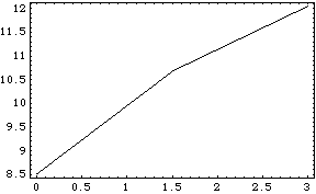
Out[61]= |  |
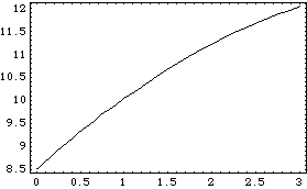
If we use TimeInterpolate to interpolate among the three points, the curve looks much smoother, but it is still a very poor representation, because there is no way for the InterpolatingFunction to know that the curvature increases as T approaches zero. Here we interpolate the shock length function with a default InterpolationOrder that is too high.

Out[62]= |  |
Here is a plot of the zeroth-order representation of shocklength.
Out[63]= |  |
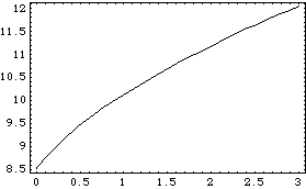
A new table of three solution rules is calculated, but this time velocity and acceleration data is included. To avoid recalculating all of the location solution points, SolveMech is passed the list of location solutions that have already been generated. This generates a new list of solution rules using the existing rules as initial guesses. The higher-order slope and curvature information contained in acctab is automatically included in the new InterpolatingFunction object returned by TimeInterpolate. Again, we interpolate the shocklength function. Here is a plot of the second-order representation of shocklength.
Out[66]= |  |
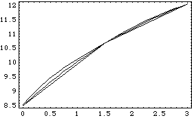
Here are the three plots shown together.
Out[67]= |  |
Interpolating SolutionsAnother method of applying interpolation is to directly interpolate the rules returned by SolveMech. SolveMech accepts the symbol Interpolation as an option name to tell SolveMech to interpolate the rules it returns. Note that SolveMech does not interpolate variables that are constant. An option for SolveMech. Because the Solution -> Acceleration option is given in the following example, the InterpolatingFunction objects returned contain slope and curvature information from the velocity and acceleration solutions. Here is a set of interpolated solution rules.
Out[69]= | 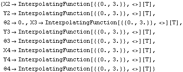 |
Here is another plot of shocklength.
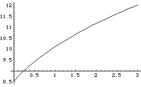
Out[70]= |  |
|