When a constant diagonal scaling compensator that gives acceptable levels of diagonal dominance over the bandwidth of interest cannot be found, a dynamic diagonal scaling compensator can often be determined that will result in diagonal dominance over all frequencies of interest (Munro (1985)). This is done by determining simple scalar rational functions that approximate well the amplitude behaviors of the elements of the appropriate Perron-Frobenius eigenvector with frequency. The resulting dominance ratios will depend on the goodness of the fit. The function PerronFrobeniusEigenvectorPlot displays the amplitude behavior of the elements of the right and left Perron-Frobenius eigenvector for the direct and inverse systems, respectively. | PerronFrobeniusEigenvectorPlot[system] |
| | plot the amplitude behavior of the elements of the Perron-Frobenius right eigenvector for the object system |
| PerronFrobeniusEigenvectorPlot[system, {w, wmin, wmax}] |
|
| | display the plot for frequency w running from wmin to wmax |
Creating the Perron-Frobenius eigenvector plot for direct systems. | PerronFrobeniusEigenvectorPlot[InverseSystem[system]] |
| | plot the amplitude behavior of the elements of the Perron-Frobenius left eigenvector for the object system |
| PerronFrobeniusEigenvectorPlot[InverseSystem[system], {w, wmin, wmax}] |
|
| | display the plot for frequency w running from wmin to wmax |
Creating the Perron-Frobenius eigenvector plot for inverse systems. Make sure the application is loaded. This is the two-input, two-output transfer-function object, considered in Section 5.3.1. | Out[3]= |  |
These are the Perron-Frobenius eigenvector plots for this system. 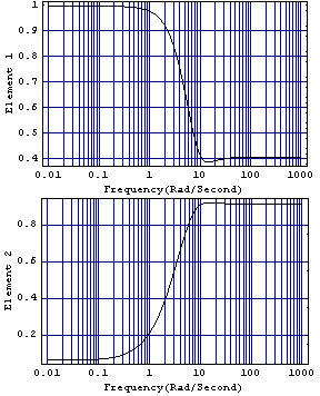
These plots show that the elements of the Perron-Frobenius eigenvector vary considerably with frequency, which explains why a constant scaling compensator designed with the function PerronFrobeniusCompensator in Section 5.3.1 failed to achieve diagonal dominance over the bandwidth of interest. The same function PerronFrobeniusCompensator can also find a dynamic diagonal scaling compensator by approximating the amplitude behaviors of the elements of the right Perron-Frobenius eigenvector of the direct system (or the left Perron-Frobenius eigenvector of the inverse system), over the desired frequency range. For this purpose, PerronFrobeniusCompensator internally calls the function NonlinearRegress. Consequently, PerronFrobeniusCompensator accepts the options of NonlinearRegress and passes them along to their destination. | PerronFrobeniusCompensator[system, {wmin, wmax}, n] |
| | calculate a Perron-Frobenius dynamic compensator for the object system, for frequency  running from wmin to wmax,with numerators and denominators of order n running from wmin to wmax,with numerators and denominators of order n |
| PerronFrobeniusCompensator[system, {wmin, wmax}, { n, d}] |
| | calculate a Perron-Frobenius dynamic compensator for system, with all numerators and denominators of the same order {n, d} |
| PerronFrobeniusCompensator[system, {wmin, wmax}, {{n1, d1}, {n2, d2}, ...}] |
|
| | calculate a Perron-Frobenius dynamic compensator for system,
with numerators and denominators of orders {{n1, d1}, {n2, d2}, ...} |
The Perron-Frobenius dynamic compensator functions. This determines two dynamic compensators each with numerator and denominator of order 3. On your computer system, the result may be numerically different (with the default set of options), but the approximation should still be good. You may achieve a result closer the one below by supplying a different value of the option Method (for example, using Method -> QuasiNewton) and changing AccuracyGoal, WorkingPrecision, and/or other options. | Out[6]= |  |
You can assess the goodness of these approximations with respect to the behavior of the elements of the Perron-Frobenius eigenvector, over a range of frequencies, by first using the function MagnitudeFrequencyPlot to obtain the amplitude behavior of the dynamic elements on the diagonal of this compensator, with frequency. These responses can then be compared with those of the eigenvector elements. | MagnitudeFrequencyPlot[comp] |
| | plot the amplitude behavior of the elements of the Perron-Frobenius compensator comp |
| MagnitudeFrequencyPlot[comp, {w, wmin, wmax}] |
|
| | plot the amplitude behavior for frequency w running from wmin to wmax |
Creating a magnitude frequency-response plot. Since plots of constant responses usually provide little useful information, MagnitudeFrequencyPlot drops these by default. You can use the option DropConstant to change this behavior. | option name | default value | | | DropConstant
| True | whether to drop constant responses |
Option specific to MagnitudeFrequencyPlot. This determines the amplitude behavior of the diagonal elements of this compensator. 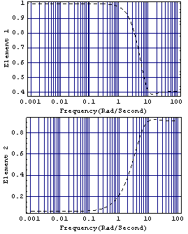
This compares the behavior of the elements of the Perron-Frobenius eigenvector and the diagonal elements of the compensator. 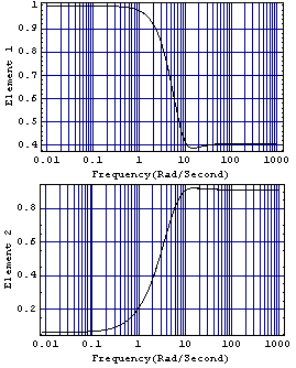
The solid-line plots are the characteristics of the elements of the Perron-Frobenius eigenvector concerned, and the dashed-line plots are the amplitude behaviors of the approximations determined as comp33. Clearly, the fits obtained are very good using these third-order compensators, and you would accordingly expect the dominance ratios achieved in both rows to be almost identical and also to be close to those predicted by the Perron-Frobenius eigenvalue plot. This applies the compensator to the system. These are the resulting dominance ratios. 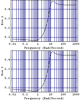
This is the resulting Nyquist array. 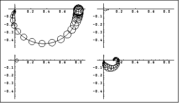
This scales up row 2 of the Nyquist array to give a more clear plot. Here is the resulting Nyquist array. 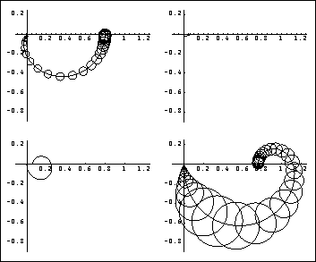
Clearly, by changing the dynamics of the system, the desired diagonal dominance has been achieved in both diagonal elements of the Nyquist array. The shape of element {2, 2} has changed most significantly. |