When the Perron-Frobenius scaling approach is not able to produce a diagonal scaling compensator that achieves diagonal dominance, the designer has to consider the use of a nondiagonal matrix compensator. One such approach, which was initially developed by Hawkins (1972) for use with inverse systems, is to determine the inverse compensator  as the best, in a least-mean-squares sense, wholly real matrix that most nearly diagonalizes the system as the best, in a least-mean-squares sense, wholly real matrix that most nearly diagonalizes the system  at some frequency s = j at some frequency s = j (Rosenbrock (1974), and Patel and Munro (1982)). In this approach, the inverse compensator (Rosenbrock (1974), and Patel and Munro (1982)). In this approach, the inverse compensator  is determined row by row, as necessary, so that for row j is determined row by row, as necessary, so that for row j is made as small as possible, subject to the constraint that This leads to an eigenvalue/eigenvector problem, where a different frequency can be chosen for each row of  . The function PseudodiagonalizingCompensator implements this approach. Note that the constraint in Eq. (5.NumberedEquationPseudodiagonalizing Compensator constant) does not prevent the diagonal term . The function PseudodiagonalizingCompensator implements this approach. Note that the constraint in Eq. (5.NumberedEquationPseudodiagonalizing Compensator constant) does not prevent the diagonal term  from becoming very small, or vanishing altogether, even though the resulting row of from becoming very small, or vanishing altogether, even though the resulting row of  is diagonal dominant. If the resulting diagonal terms are very small, but not equal to zero, the option Method is diagonal dominant. If the resulting diagonal terms are very small, but not equal to zero, the option Method  QNorm ensures that the compensator is adjusted so that all the diagonal terms QNorm ensures that the compensator is adjusted so that all the diagonal terms  . The default value of this option is Method KNorm, which corresponds to the constraint given in Eq. (5.NumberedEquationPseudodiagonalizing Compensator constant). . The default value of this option is Method KNorm, which corresponds to the constraint given in Eq. (5.NumberedEquationPseudodiagonalizing Compensator constant). | PseudodiagonalizingCompensator[InverseSystem[system] ] |
| | calculate a pseudo-diagonalizing compensator for all rows of the inverse system, at zero frequency |
| PseudodiagonalizingCompensator[InverseSystem[system], w] |
| | calculate a pseudo-diagonalizing compensator at the frequency w |
| PseudodiagonalizingCompensator[InverseSystem[system], {w1, w2, ..., wk}, {r{1}, r{2}, ..., rk}] |
|
| | calculate a pseudo-diagonalizing compensator at the frequencies {w1, w2, ..., wk} for rows {r{1}, r{2}, ..., rk}, where k is less than or equal to the number of rows of the inverse system |
The pseudo-diagonalizing compensator functions for inverse systems. For direct systems, since Q(s) = G(s) Kp, the function PseudodiagonalizingCompensator, which computes Kp, operates on the columns of G(s). | PseudodiagonalizingCompensator[system] |
| | calculate a pseudo-diagonalizing compensator for all columns of system, at zero frequency |
| PseudodiagonalizingCompensator[system, w] |
| | calculate a pseudo-diagonalizing compensator for all columns of system, at the same frequency w |
| PseudodiagonalizingCompensator[system, {w1, w2, ..., wk}, {c{1}, c{2}, ..., ck}] |
|
| | calculate a pseudo-diagonalizing compensator at the frequencies {w1, w2, ..., wk} for columns {c{1}, c{2}, ..., ck}, where k is less than or equal to the number of columns of system |
The pseudo-diagonalizing compensator functions for direct systems. Make sure the application is loaded. Consider a two-input, two-output multivariable system described by the transfer-function model. | Out[3]= | 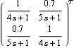 |
The time responses of the open-loop system, when a unit step is applied to each input separately, show that there is considerable interaction present in the system. 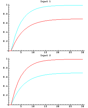
Here is the inverse-system Nyquist array of this system, with the Gershgorin circles for row dominance superimposed on the diagonal terms. 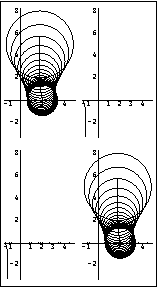
While the system is diagonal dominant, since none of the Gershgorin circles enclose the origin of their respective plots, you can further improve the overall diagonal dominance of this system by designing a pseudo-diagonalizing compensator. Here is a compensator determined by applying the pseudo-diagonalization method to both rows of the inverse-system Nyquist array at zero frequency. | Out[7]= | 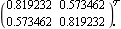 |
This applies the pseudo-diagonalizing compensator to the system. | Out[9]= | 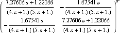 |
The compensator has completely eliminated the interaction in both rows of the system at zero frequency. 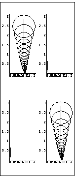
As you are using the inverse-system Nyquist array, the effect of additional feedback loop gains on the interaction present in the system can be assessed by superimposing the Ostrowski circles on the diagonal terms of the inverse-system Nyquist array. As can be seen from the Ostrowski circles, further significant reduction in the interaction in both loops can be achieved by closing the loops, for example, with unity feedback. 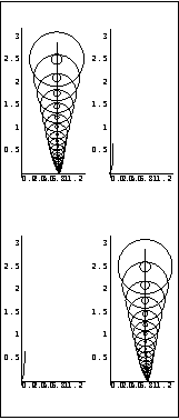
As this system responds well when the same pseudo-diagonalization frequency is used for both rows, due to the symmetric form of the system model, a frequency of 0.4 rad/s produces a good uniform reduction in the Gershgorin circles for both diagonal elements of the inverse-system Nyquist array. Pseudo-diagonalization at other frequencies produces a less uniform reduction in the Gershgorin circles. This applies the pseudo-diagonalization method to both rows at = 0.4 rad/s. | Out[13]= | 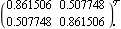 |
This is the resulting forward-path transfer-function matrix. | Out[15]= | 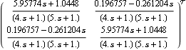 |
Here is the resulting inverse-system Nyquist array with Gershgorin row dominance circles, and Ostrowski circles for additional loop gains {1, 1}. 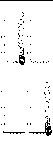
Now, both the low-frequency and high-frequency interactions in the system have been significantly reduced in both loops. The very small Ostrowski circles indicate that most of the interaction in the system will be eliminated when both feedback loops are closed with unity feedback. This is the explicit form of the compensator. | Out[18]= | 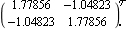 |
This closes the feedback loops. Here is a simulation of the resulting closed-loop system. 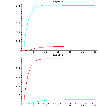
Here are two PI single-loop compensators that remove the steady-state error and further reduce the interaction. | Out[22]= | 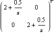 |
This is the new closed-loop system. This calculates the new closed-loop system transfer-function matrix. Here is its simulated response. 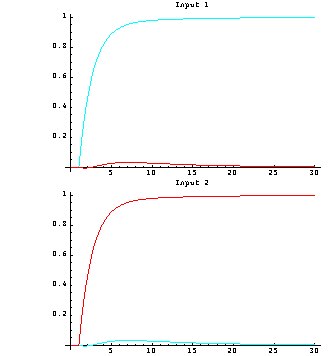
The introduction of the two additional PI action single-loop controllers has clearly corrected the steady-state errors in the primary outputs, and has also removed any remaining steady-state interaction in both outputs due to the presence of the integrators. The resulting closed-loop control system has the simple structure shown in Figure 5.1, where Kp is the constant compensator designed using the pseudo-diagonalization approach and k1(s) and k2(s) are the two single-loop PI compensators. This is the overall forward-path compensator designed for this system using the inverse-system Nyquist array. | Out[27]= | 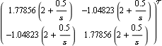 |
|
