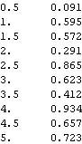
1.4.1 Plotting the DataThe first thing to do in analyzing time series data is to plot them since visual inspection of the graph can provide the first clues to the nature of the series: we can "spot" trends, seasonality, and nonstationary effects. Often the data are stored in a file and we need to read in the data from the file and put them in the appropriate format for plotting using Mathematica. We provide several examples below. Example 4.1 As an illustrative example of how to read in data from a file, let us suppose that we have a file called file1.dat in the directory TimeSeries/Data. (Note that specification of files and directories depends on the system being used.) The file consists of two columns of numbers. The numbers in the first column are the times when the observations were made and those in the second column are the outcomes of observations, that is, the time series. We can look at the contents of file1.dat using FilePrint. We load the package first. This displays the contents of the file file1.dat in the directory TimeSeries/Data. We use the ReadList command to read in these numbers and put them in a list. We read in the time series data from the file file1.dat. The specification {Number, Number} in ReadList makes each entry in the list a list of two numbers {t, xt}. | Out[3]= |  |
Now data1 defined above is in the right format for ListLinePlot. We plot the data using ListLinePlot. | Out[4]= | 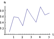 |
We can check if the data were in fact taken at equally spaced intervals by doing the following. First extract the time coordinates. The time coordinates are the first element of each data point. | Out[5]= |  |
Now take the differences of adjacent time coordinates and see if they give the same number. The differences are the same. | Out[6]= |  |
So we see that in this case the data were indeed taken at constant time intervals. Since we have assumed all along that the data are taken at equally spaced time intervals, it is often convenient to drop the time coordinate and consider just the time series. All time series data to be input to time series functions should be in the form {x1, x2, ... , xn} where xi is a number for a scalar time series and a list, xi={xi1, xi2, ... , xim}, for an m-variate time series. We can cast the above data in the form appropriate for input to time series functions by taking the second (i.e., the last) entry from each data point. This extracts the time series. | Out[7]= |  |
Now the data are in the right form to be used in time series functions. If we plot the above data using ListLinePlot we will get the same plot as before except (a) the origin of time will have been shifted and (b) it will be in different time units with the first entry in data corresponding to time 1, and the second to time 2, and so on. Here is the time plot for the same series. | Out[8]= | 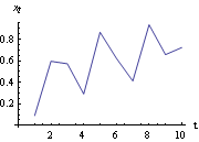 |
Example 4.2 Often the time series data are stored in a file without the time coordinates, as in the case of the lynx data in the file lynx.dat in the directory TimeSeries/Data. The file contains a series of numbers separated by blanks. This reads in the contents of the file lynx.dat in the directory TimeSeries/Data. It is convenient to use the Mathematica function Short to find out if the data are in the appropriate format without printing out all the numbers. This gives the short form of lynxdata. | Out[10]//Short= | 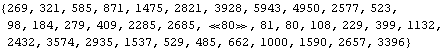 |
We can plot lynxdata directly using ListLinePlot as we have demonstrated in the previous plot. On the other hand, if we want the time plot to show the real times at which the data were taken, we can reverse the above procedure of transforming data1 to data. Suppose the data were taken from time t1 to tn in intervals of  t t, Range[t 1, tn, deltat] will generate a list of all the times at which data were taken. If t is omitted the default value of 1 is assumed. In our lynx example, the data were taken annually from the year 1821 to the year 1934. This combines the time series with the time coordinates. We use Short to display data1. | Out[12]//Short= | 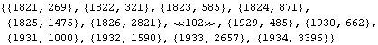 |
Now if we plot data1 using ListLinePlot the horizontal axis corresponds to the "real" time. Here is the time plot of the lynx data. | Out[13]= | 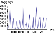 |
Example 4.3 The file file2.dat has a set of bivariate data with column 1 containing series 1 and column 2 containing series 2, separated by commas. Again we employ ReadList to read the data. We read in the data from file2.dat. We have used the option RecordSeparators -> "," because of the presence of commas between the numbers. To convert data1, which is now a long list of numbers, into the correct time series data format we put every pair of numbers into a list using Partition. We use Partition to put the data in the right form for a multivariate series. Here are a few elements of data. | Out[16]= |  |
We see that data is a bivariate time series of length 100. Again it is in the correct format of the form {x1, x2, ... , xn} with the ith entry xi being a list of length 2. To extract the ith time series from multivariate data we can use data[[All,i]]. Here are the plots of the two series of the bivariate series data. This is the time plot of series 1 of the bivariate series in file2.dat. | Out[17]= | 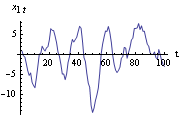 |
This is the time plot of series 2 of the bivariate series in file2.dat. | Out[18]= | 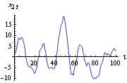 |
|