1.8.2 The Spectra of Linear Filters and of ARMA ModelsIn this section we will derive the spectrum of a filtered process and of an ARMA process from the definitions given in Section 1.8.1. We will assume that the appropriate transformations have been made to render the process under consideration zero-mean and stationary. Spectrum of a Linear Filtered ProcessWe have introduced the concept of a time-invariant linear filter in Section 1.4. Now we want to look at the effect of filtering on the spectrum of a process. Let {Yt} be a stationary, zero-mean process with spectrum fY( ) ) and Xt=  jYt-j jYt-j. The (constant) filter weights { j} j} satisfy    j j < < . Using the definitions of covariance function and ( 8.1), it is straightforward to show that the spectrum of the filtered process {Xt} is given by As an exercise let us write a little program to calculate the power transfer function T( ) ) of a given linear filter. We assume that only a finite number of filter weights are nonzero ( i.e.,  j=0 j=0 for  j j larger than a positive number M). With this assumption, as we have pointed out before, we can always treat a linear filter as a causal (or one-sided) one ( i.e.,  j=0 j=0 for j<0) since doing so only amounts to a "time shifting" in time domain or an extra phase factor in the transfer function, and it leaves the power transfer function invariant. Therefore, the filter weights can be input in the form "weight"={ 0, 0,  1, 1,  2, ... , 2, ... ,  M} M}. The transfer function for a list of weights weight can be defined as Table[E^(-I  j),{j, 0, Length[weight] - 1}].weight Calling the expression for the transfer function tf, the power transfer function can be defined as tf * (tf /. a_Complex -> Conjugate[a]) Using the above two lines, we can define a Mathematica function called powertransferfunction, which computes   (e-i (e-i ) ) 2 2 given the filter weights { j} j} and the frequency variable  as arguments. We define a function to calculate the power transfer function. Example 8.2 Find the power transfer function of a simple moving average. A simple moving average of order M is a linear filter of weights  j=1/M j=1/M for j=0, 1, ... , M-1 and  j=0 j=0 otherwise. We use the function defined above to find the power transfer function of the simple moving average filter of order 5. This is the power transfer function of a moving average of order 5. | Out[3]= |  |
We plot the above power transfer function. | Out[4]= | 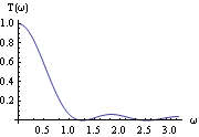 |
The power transfer function of the filter has a maximum at  =0 =0 and is rather small at "high" frequencies. Since the spectrum of the filtered process is the original spectrum multiplied by this function, we see that the effect of the moving average is to suppress the high frequency (short time) part of the spectrum in the original process and retain the low frequency (long time) spectrum. The kind of filter is called a low-pass filter. This is why we can use the moving average to eliminate short time fluctuations and, thus, estimate long-term trends. Spectrum of an MA("q") ProcessAn MA( q) process can be thought of as a white noise process {Zt} passed through a linear filter of weights {1,  1, 1,  2, ... , 2, ... ,  q} q}. From ( 8.3) an MA( q) process has the spectrum Spectrum[model,  ] ] gives the spectrum of an ARMA type of model as a function of frequency  and its code resembles the above demonstration program. (We can also obtain the same MA spectrum by finding the power transfer function and multiplying it by the white noise spectrum.) Example 8.3 Find the power spectrum of an MA(1) process Xt=Zt+ 1Zt-1 1Zt-1. This gives the spectrum of an MA(1) process. | Out[5]= |  |
We see that the spectrum of an MA(1) process is the otherwise flat white noise spectrum multiplied by a weight function (power transfer function), which depends on  . Since cos is monotonically decreasing for  in [ 0,  ], as the frequency  increases f( ) ) decreases for positive  1 1 and increases for negative  1 1. Also since the covariance function at lag 1,  (1) (1), is  1 1, a negative  1 1 can cause the series to fluctuate rapidly and we expect large contributions to the variance at high frequencies. This is indeed the case as we see in the following graph. Here is the MA(1) spectrum for  1=-0.8 1=-0.8 and  2=1 2=1. % /. { -> 1, -> 1,  1 -> -0.8} 1 -> -0.8} is used to replace s and t1 in the above expression with the corresponding values. | Out[6]= | 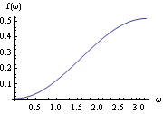 |
As an exercise we can plot spectra of different MA models just to develop some intuition. For example, let us find and plot the spectrum for an MA(2) model with  1=-0.5 1=-0.5 and  2=0.9 2=0.9. This calculates the spectrum of the MA(2) model. Here is the plot of the spectrum. Evaluate is used inside the Plot to speed up generation of the plot. | Out[8]= | 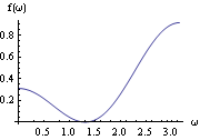 |
Spectra of AR("p") and ARMA("p", "q") ProcessesSimilarly, using ( 8.3) and writing Zt= (B)Xt (B)Xt, the spectrum of an AR( p) process is simply given by fZ( )= )=  (e-i (e-i ) ) 2fX( 2fX( ) ) or Example 8.4 Find the spectrum of an AR(1) process Xt- 1Xt-1=Zt 1Xt-1=Zt. This is the spectrum of an AR(1) model. | Out[9]= |  |
Again the power spectrum is monotonic in  and, depending on the sign of  1 1, the power is concentrated at either low or high frequencies. For  1=0.7 1=0.7 and  2=1 2=1 we plot the spectrum. Here is the spectrum of the AR(1) model with  1=0.7 1=0.7. | Out[10]= | 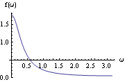 |
In general the spectrum of an AR( p) process is not monotonic and depending on the signs of the AR coefficients the spectrum can assume different shapes. We calculate the spectrum of an AR(2) process with  1=1 1=1 and  2=-0.5 2=-0.5. Here is the plot of the above spectrum. | Out[12]= | 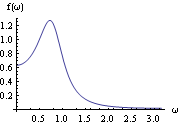 |
This is often called a rational spectrum. AR and MA spectra are special cases of this spectrum when  (x)=1 (x)=1 and  (x)=1 (x)=1, respectively. Example 8.5 Calculate the spectrum of an ARMA( 1, 1) process. This gives the spectrum of an ARMA( 1, 1) process. | Out[13]= |  |
Note that the noise variance has been set to 1. The values of  1 1 and  1 1 determine the shape of the spectrum. Here is the plot of the spectrum with  1=-0.5 1=-0.5 and  1=0.8 1=0.8. | Out[14]= | 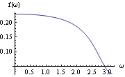 |
Example 8.6 Here we give an example of spectrum of a seasonal model. Consider the model (1- 1B)(1- 1B)(1- 1B6)Xt=Zt 1B6)Xt=Zt. It has the following spectrum. This is the spectrum of the given seasonal model. | Out[15]= |  |
This is the plot of the spectrum. | Out[16]= | 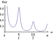 |
We have used the option Ticks -> {{0,  /3, 2 /3, 2 /3, /3,  }, Automatic} }, Automatic}, which yields tick marks at specified points along the abscissa and puts them automatically along the ordinate. This multiplicative seasonal process can be thought of as two successive linear filters being applied to a white noise process, and the spectrum is the product of the two corresponding power transfer functions and the white noise spectrum. The seasonal part of the spectrum has an  dependence through cos6 . Since cos6 =1 =1 for  =0, =0,  /3, 2 /3, 2 /3 /3, and  , the seasonal part of the spectrum reaches its maximum value at these frequencies for  1>0 1>0. This spectrum is again weighted by the monotonically decreasing ordinary AR spectrum resulting in the final shape of the spectrum we see above. |