1.8.5 Spectrum for Multivariate Time Series The definition of the spectrum of multivariate time series is similar to that in the univariate case except now we deal with a spectrum matrix (spectral density matrix) f( ) ) given by (see ( 8.1)) where  (k) (k) is the covariance matrix defined in Section 1.2.5 (see ( 2.11)). The ith diagonal element of f(), fii(), is the (auto)spectrum of the time series i and the off-diagonal element fij()=1/(2 ) )  ij(k)e-ik ij(k)e-ik ( i≠j) is called the cross spectrum (cross spectral density function) of time series i and j. Note that as in the univariate case, f() is 2-periodic. However, since ij(k) and ij(-k) need not be the same the cross spectrum fij() is in general complex and it can be written as Various spectra relating to the cross spectrum can be defined from ( 8.13). The real part of the cross spectrum, cij(), is called the cospectrum, and the negative imaginary part, qij(), the quadrature spectrum; the amplitude of the cross spectrum,  ij()= ij()= fij() fij() is called the amplitude spectrum and the argument,  ij() ij(), the phase spectrum. Two other useful functions are the squared coherency spectrum (some authors call it coherence) and gain function of time series i and j, and they are defined by  and Gij()=fij()/fi(), respectively. Although these functions are defined separately due to their different physical interpretations, all the information is contained in our basic spectrum ( 8.12), and we will see that it is a simple matter to extract these quantities once the spectrum f() is known. Spectra of Linear Filters and of ARMA ModelsThe transfer function of a linear filter in multivariate case is defined similarly except that now the filter weights { j} j} are matrices. Equation ( 8.3) is generalized to and a function implementing ( 8.14) can be easily written to get the spectrum of a filtered process. This will be left as an exercise for the diligent reader. The ARMA spectrum can be derived as in the univariate case using ( 8.14); it is given by and the same function Spectrum[model, ] applies to the multivariate case. Example 8.10 Here is an example of the spectrum of a multivariate ARMA( 1, 1) process. This defines a bivariate ARMA( 1, 1) model. | Out[41]= | 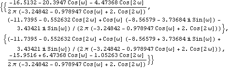 |
Here is the cospectrum of the above ARMA( 1, 1) model. | Out[42]= |  |
If we only want to see the plot of the spectrum and do not need the explicit function form, we can simply use the function Re to extract the real part of fij(). This is the plot of the cospectrum. | Out[43]= | 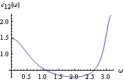 |
Similarly we can get other spectra. Here is the plot of the quadrature spectrum. | Out[44]= | 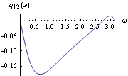 |
Here is the plot of the squared coherency. | Out[45]= | 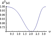 |
Various other spectra can be plotted using the built-in Mathematica functions Abs, Arg, etc. Estimation of the SpectrumWe can estimate the spectrum of an ARMA process by fitting an m-variate ARMA model to m-variate data and using Spectrum[model, ] to get the estimated spectra. The sample spectrum of a multivariate process is again given by ( 8.5) with the sample covariance matrix  in place of univariate sample covariance function  . As in the univariate case, the function Spectrum[data] gives the sample spectrum of m-variate data at frequencies j=2j/n for j=0, 1, ... , n-1, and its output is { } } where  is an m m m matrix. Again, the function normalizedspectrum defined earlier (see Example 8.7) can be used to estimate the normalized spectrum in the multivariate case. Example 8.11 Here is the sample spectrum of a bivariate time series data of length 100 generated from the ARMA( 1, 1) model used in Example 8.10. The random number generator is seeded. This generates the time series. This calculates the sample spectrum. And from this sample spectrum, we can obtain all the other spectra. For example, the cospectrum can be obtained by extracting the (1, 2) component of the sample spectrum matrix and taking its real part. Here we plot the sample cospectrum. | Out[49]= | 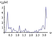 |
To smooth the spectrum we proceed as in the univariate case. SmoothedSpectrumL[cov, window, ] and SmoothedSpectrumS[spec, window] are used to get the smoothed spectrum matrix  and matrices  for j=0, 1, ... , n-1, respectively. They are defined in ( 8.7) and ( 8.8) with  and  now replaced by the sample spectrum matrix and sample covariance matrix. Matrix weights can also be used. For example, W and  in "window"={W(0), W(1), ... W(M)} and "window"={(0), (1), ... (M)} can be matrices so that different components do not have to be smoothed with the same window. The (i, j) component of the spectrum will be smoothed according to where W(-k)=W (k) (k) and (-k)=(k) are assumed throughout. If scalar weights are entered, all the components will be smoothed using the same given weights. Example 8.12 Smooth the spectrum of Example 8.11 using the Bartlett window. We first calculate the sample covariance function. This gives the smoothed spectrum using the Bartlett window. This is the plot of the smoothed cospectrum. | Out[52]= | 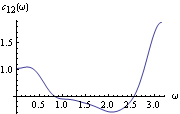 |
Next we look at the smoothed cospectrum using the Daniell window. This gives the smoothed spectrum using the Daniell window. This is the plot of the cospectrum. | Out[54]= | 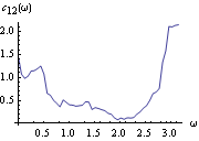 |
For comparison we display the two smoothed cospectra together with the theoretical cospectrum (see plot0 in Example 8.10). This displays the three cospectra together. | Out[55]= | 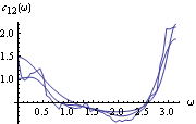 |
It is a simple matter to get estimates for other spectra once  is known. For example, as we have demonstrated, the cospectrum is simply the real part of the appropriate component of the spectrum and it is trivial to extract it using the Re and Map functions. You can also define your own functions to extract different spectra. For example, you can define the following function to get the squared coherency between series i and j. Note here that spec should be a smoothed discrete spectrum so that the denominator will not be zero at =0. |
