Hyperelastic Model Comparison
| Introduction | FEM uniaxial test |
| Uniaxial test data generation | Conclusion |
| Model fitting | Nomenclature |
| Analytical comparison | References |
The following examples compare different hyperelastic models with a brief discussion about picking the model that best fit your experimental data.
Introduction
Selecting the correct hyperelastic model for a specific material requires considering several factors, including the material's mechanical behavior, available experimental data, and the intended application.
Experimental data is crucial for selecting an appropriate hyperelastic model. Mechanical tests, such as uniaxial tension, compression, or shear tests, are conducted to measure the material's stress-strain response under different loading conditions.
For soft tissue, for example, uniaxial tensile testing is commonly used gain experimental data due to the relatively simple and controlled experimental setup. The specimens are subjected to controlled tensile forces in a single direction, allowing for precise measurements and analysis. The uniaxial loading condition ensures that the stress and strain are predominantly applied along one axis, simplifying the analysis of the mechanical behavior. Displacement data is recorded as a function of force between the grips of the testing machine.
More information on experimental tests is given in the Hyperelasticity monograph.
We load the finite element context for additional functions used in the remainder of the tutorial.
Uniaxial test data generation
In order to fit the hyperelastic model of interest we need experimental data describing the material behavior aforementioned. In the following section, a uniaxial tensile test is considered to collect data representing the stress-stretch relation. To avoid to have to go to the lab, the experimental data is generated virtually. For this we use an analytically expressing the relation between stress and stretch due to a specific constitutive behavior.
As expressed in the Hyperelasticity monograph, the uniaxial stress is related to the strain energy ![]() and the stretch
and the stretch ![]() as:
as:
To generate virtual experimental data a constitutive model need to be selected. For instance, we use a Yeoh model, that combine simplicity of a polynomial function while still showing a well marked non-linear behavior. Clearly, a different constitutive model or different material parameters change the experimental data and consequently all the following comparison results.
We start by inserting the Yeoh strain energy into the uniaxial stress expression and get to:
where ![]() is the first strain invariant
is the first strain invariant ![]() .
.
Due to the incompressibility constraint ![]() the second and third principal stretches are related to the main principal stretch as
the second and third principal stretches are related to the main principal stretch as ![]() . The first strain invariant can then be expressed with respect to the main stretch
. The first strain invariant can then be expressed with respect to the main stretch ![]() as:
as:
In the following experimental data is generated as stress-stretch relation with the addition of noise to simulate the imperfection of real data. The noise added also shows how the performed material model fitting can be affected by data quality.
It is important to realize that in this example two different data ranges data are considered. The data from the experiment is typically over a larger range than the data used for the actual model fit. This is because we would like to create an as accurate fit as possible and this is done by only fitting the data range of interest and not going beyond that.
Although the virtual experimental data reaches a maximal stretch of ![]() , the fitting of the models is performed on a restricted range. This is later to show how models' accuracy depends on the chosen data range. In fact, as we will see later, models that perform similar in a certain range can show large differences when leaving this range.
, the fitting of the models is performed on a restricted range. This is later to show how models' accuracy depends on the chosen data range. In fact, as we will see later, models that perform similar in a certain range can show large differences when leaving this range.
To emphasize this once more, the choice of the maximal stretch used for the model fitting here is arbitrary. When performing a fit with real data one should take into consideration the expected stretch in the actual application and choose the data range based on that.
Model fitting
In the following step a hyperelastic material model fit is created based on the uniaxial tensile test data. Typically the data is obtained from a series of experiments or, like in our case, we have created virtual material data. In this section several incompressible hyperelastic material models are fitted to the same data.
By considering the strain energy ![]() of a specific model it leads to an analytical expression from which it possible to identify the material parameters for the desired constitutive model thought a fitting procedure.
of a specific model it leads to an analytical expression from which it possible to identify the material parameters for the desired constitutive model thought a fitting procedure.
For each model, the material parameter identification procedure is the same: First, the strain energy is derived with respect to the first and second invariants to compute the uniaxial stress ![]() , as expressed in eqn (1). Then, a numerical fitting is performed to search for the optimal material parameters to represent the test data.
, as expressed in eqn (1). Then, a numerical fitting is performed to search for the optimal material parameters to represent the test data.
Neo-Hookean
The strain energy for the incompressible neo-Hookean model is:
For the uniaxial test the stress from eqn (2) reads:
Mooney-Rivlin 2 parameters
The strain energy for the incompressible 2 parameters Mooney-Rivlin model is:
Where ![]() and
and ![]() are the two material parameters.
are the two material parameters.
A consistent fitting also requires an additional constraint, ![]() , in order to satisfy the positiveness of the strain energy. The constraint ensures numerical material stability.
, in order to satisfy the positiveness of the strain energy. The constraint ensures numerical material stability.
For the uniaxial test the stress from eqn (3) reads:
Mooney-Rivlin 5 parameters
The strain energy for the incompressible 5 parameters Mooney-Rivlin model is:
So, for the uniaxial test the stress from eqn (4) reads:
Mooney-Rivlin 9 parameters
The strain energy for the incompressible 9 parameters Mooney-Rivlin model is:
For the uniaxial test the stress from eqn (5) reads:
Arruda-Boyce
The strain energy for the incompressible Arruda-Boyce model is:
Where ![]() and
and ![]() are the two material parameters of the model while the
are the two material parameters of the model while the ![]() are the numerical coefficients from the Taylor expansion:
are the numerical coefficients from the Taylor expansion:
For the uniaxial test the stress from eqn (6) reads:
Gent
The strain energy for the incompressible Gent model is:
Where ![]() and
and ![]() are the two material coefficients.
are the two material coefficients.
For the uniaxial test the stress from eqn (7) reads:
Yeoh
The strain energy for the incompressible Yeoh model is:
For the uniaxial test the stress from eqn (8) reads:
Analytical comparison
The following section compares the different fitted models. By focusing on the fitting range the Yeoh, Mooney-Rivlin Five and Mooney-Rivlin Nine appear to best fit the available data due to their polynomial nature. Instead, the simple Mooney-Rivlin, Arruda-Boyce and Gent appear to be reduced to linear-like behaviour much like the neo-Hookean model.
The model behaviour is strictly confined to the fitting range. When using the models beyond a stretch of ![]() the majority of the models will diverge from the remaining experimental data, while the Mooney-Rivlin Five and the Yeoh model remain close to the expected range of stress. The models have been specially been fitted to only a small part of the data,
the majority of the models will diverge from the remaining experimental data, while the Mooney-Rivlin Five and the Yeoh model remain close to the expected range of stress. The models have been specially been fitted to only a small part of the data, ![]() to showcase their behaviour beyond that stretch and to make a point to be careful to not use a model beyond it's validity which is given by the fitting range. A fit over the entire data range would lead to different results.
to showcase their behaviour beyond that stretch and to make a point to be careful to not use a model beyond it's validity which is given by the fitting range. A fit over the entire data range would lead to different results.
FEM uniaxial test
In the following section several FEM analysis are implemented to show numerical difference between the models. The following analysis represent an uniaxial tensile test performed over a sample made of soft tissues showing an hyperelastic behaviour. The previously fitted model are used to describe the material.
3D model
The uniaxial tensile test is a standardized procedure to mechanically test material. Here, a rectangular shaped sample is pulled by one extremity. We first show a full 3D model in this section. In order to reduce computational complexity a subsequent section will make use of a 2D model to reduce the computational complexity.
To generate a mesh for a geometry of this topological structure, where one dimension (thickness) is much smaller than the other ones, requires a large number of elements. This is mainly because of the necessity of having a sufficient number of elements in the smaller (thickness) layer, forcing the elements size to be very small with respect to the structure size.
The reason to use at least 3 layers of elements in the thickness direction with solid elements is mainly due to two aspect: first, to accurately capture stress gradients in the thickness direction and, secondly, to capture the geometrical behaviour of the structure under tension. For a layer made up of a single element a plane stress formulation might be better suited. Furthermore, the overall structure may results stiffer than expected.
The specimen is deformed up to 120%. However, the right hand side was not represented as a clamped boundary. Here we simply applied the force on the boundary and so it shows a highly deformed extremity.
To better represent the experimental procedure, the usage of a clamp, we model the clamped area differently: The clamping area of the specimen should remain in a nearly undeformed state because it is held fixed inside the clamp, which is what is pulled. To achieve that behaviour, we can change the material property of the specimen to be much stiffer in area where the clamp is applied as model of the clamp. This addition will concentrate the deformation in the central side of the specimen leading to more accurate results.
This addition allows also to concentrate the deformation in the central side of the specimen leading to more accurate results. Also, three lines of elements should be used in the thickness to obtain accurate results and this increases the model size. A first representation of the model could be obtained with a bi-dimensional representation.
Comparison in 2D
By reducing the problem to 2D it is possible to rapidly compare several material models showing their differences. Here, the 3D uniaxial tensile test from above is reproduced in 2D. One change is made by extending the domain to allow for a special area for the clamps that pull the specimen. Clamps are stiffer and their behaviour is reproduced with neo-Hookean material model that has an at least two orders of magnitude stiffer coefficient. This procedure allows to reduce the deformation of extremity and extend the analysis over the entire specimen.
Initially, we can define mesh and boundary variables that will be used for all the material models application. Also several auxiliary functions are defined, so to define the same boundary problem, the corresponding parametric solver and the solution procedure for each different model analyzed.
In the following, the same boundary condition are used for all the simulations.
The following simulations allow to extract several information for each considered model. We would like to sample the stress-strain relation at the same steps of the parametric solution for each analysis.
The clamp regions are modeled as a high-stiffness neo-Hookean material in all simulations. This allows reducing the deformation on the extremities focusing on the specimen strain.
Due to the load directed along the ![]() direction and the specimen geometry, the most interesting strain effect are observable with the
direction and the specimen geometry, the most interesting strain effect are observable with the ![]() strain component referring to the deformation along the x direction. The same visible effect could be obtained by using the EquivalentStrain function.
strain component referring to the deformation along the x direction. The same visible effect could be obtained by using the EquivalentStrain function.
Conclusion
The numerical results reveal several differences between the models. The most evident one appears comparing models inside and outside the fitting range. For instance, Gent and Mooney-Rivlin appear similar inside the fitting range but start diverge outside as well as the Mooney-Rivlin Five, Mooney-Rivlin Nine and Yeoh.
All hyperelastic models show non-linearity, however, their intensity can vary depending on the model as well as on material parameters. Models like the neo-Hookean or Mooney-Rivlin, where the behaviour is described almost as a straight line, clearly fit the experimental data in an averaged sense but point by point the differences are high as show with the analytical comparison. In such cases, the desired model should be fitted focusing not only on the experimental data range but also on the stress-strain ranges expected in the applications.
Another difference in behaviour is shown in an initial stiffness of the specimen for the more linear models, like neo-Hookean compared to more nonlinear models like Yeoh. The material models have regions in which they are close to linear and other regions in which they are highly nonlinear. For example for the Yeoh model this is well visible in the animation where initially the deformation is larger then the neo-Hooken model deformation. Then, once a model approaches the highly nonlinear region the deformation of the Yeoh will be less because of an increased stiffness in the model. The neo-Hooken model will display a larger deformation for the same stress.
This is also the reason why a force is applied as boundary condition and not a displacement one, as it is typically done in the experimental procedure. Furthermore, such boundary load allows to obtain different deformations of the specimen between the different models. Then, differences in deformations are more easily to understand thanks to their graphical appearance with respect to differences in stresses.
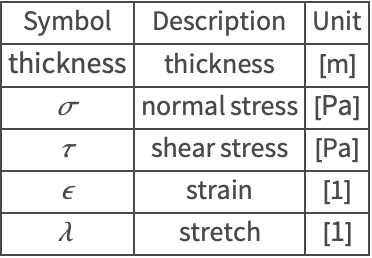
Nomenclature
References
1. Holzapfel, A.; Nonlinear Solid Mechanics; Wiley 2020; ISBN 978-0-471-82319-3