CUDA Programming
| Introduction | Writing Kernels for CUDALink |
| Writing a CUDA Kernel | Porting OpenCL to CUDA |
| Compiling for CUDA | Symbolic Code Generation |
CUDA is a general C-like programming developed by NVIDIA to program Graphical Processing Units (GPUs). CUDALink provides an easy interface to program the GPU by removing many of the steps required. Compilation, linking, data transfer, etc. are all handled by the Wolfram Language's CUDALink. This allows the user to write the algorithm rather than the interface and code.
This section describes how to start programming CUDA in the Wolfram Language.
| CUDAFunctionLoad | loads a CUDA function into the Wolfram Language |
CUDA programming in the Wolfram Language.
This document describes the GPU architecture and how to write a CUDA kernel. In the end, many applications written using CUDALink are demonstrated.
Introduction
The Common Unified Device Architecture (CUDA) was developed by NVIDIA in late 2007 as a way to make the GPU more general. While programming the GPU has been around for many years, difficulty in programming it had made adoption limited. CUDALink aims at making GPU programming easy and accelerating the adoption.
When using the Wolfram Language, you need not worry about many of the steps. With the Wolfram Language, you only need to write CUDA kernels. This is done by utilizing all levels of the NVIDIA architecture stack.

CUDA Architecture
CUDA's programming is based on the data parallel model. From a high-level standpoint, the problem is first partitioned onto hundreds or thousands of threads for computation. If the following is your computation:
OutputData = Table[fun[InputData[[i, j]]], {i, 10000}, {j, 10000}]
then in the CUDA programming paradigm, this computation is equivalent to:
CUDALaunch[fun, InputData, OutputData, {10000, 10000}]
where ![]() is a computation function. The above launches 10000×10000 threads, passes their indices to each thread, applying the function to InputData, and places the results in OutputData. CUDALink's equivalence to CUDALaunch is CUDAFunction.
is a computation function. The above launches 10000×10000 threads, passes their indices to each thread, applying the function to InputData, and places the results in OutputData. CUDALink's equivalence to CUDALaunch is CUDAFunction.
The reason CUDA can launch thousands of threads all lies in its hardware architecture. The following sections will discuss this, along with how threads are partitioned for execution.
CUDA Grid and Blocks
Unlike the message-passing or thread-based parallel programming models, CUDA programming maps problems on a one-, two-, or three-dimensional grid. The following shows a typical two-dimensional CUDA thread configuration.

Each grid contains multiple blocks, and each block contains multiple threads. In terms of the above image, a grid, block, and thread are as follows.

Choosing whether to have a one-, two-, or three-dimensional thread configuration is dependent on the problem. In the case of image processing, for example, you map the image onto the threads as shown in the following figure and apply a function to each pixel.

The one-dimensional cellular automaton can map onto a one-dimensional grid.

CUDA Program Cycle
The gist of CUDA programming is to copy data from the launch of many threads (typically in the thousands), wait until the GPU execution finishes (or perform CPU calculation while waiting), and finally, copy the result from the device to the host.

The above figure details the typical cycle of a CUDA program.
1. Allocate memory of the GPU. GPU and CPU memory are physically separate, and the programmer must manage the allocation copies.
2. Copy the memory from the CPU to the GPU.
3. Configure the thread configuration: choose the correct block and grid dimension for the problem.
4. Launch the threads configured.
5. Synchronize the CUDA threads to ensure that the device has completed all its tasks before doing further operations on the GPU memory.
6. Once the threads have completed, memory is copied back from the GPU to the CPU.
When using the Wolfram Language, you need not worry about many of the steps. With the Wolfram Language, you only need to write CUDA kernels.

Memory Hierarchy
CUDA memory is divided into different levels, each with its own advantages and limitations. The following figure depicts all types of memory available to CUDA.

Global Memory
The most abundant (but slowest) memory available on the GPU. This is the memory advertised on the packaging—128, 256, or 512 MB. All threads can access elements in global memory, although for performance reasons these accesses tend to be kept to a minimum and have further constrictions on them.
The performance constrictions on global memory have been relaxed on recent hardware and will likely be relaxed even further. The general rule is that performance is deteriorated if global memory is accessed more than once.
Texture Memory
Texture memory resides in the same location as global memory, but it is read-only. Texture memory does not suffer for the performance deterioration found in global memory. On the flip side, only char, int, and float are supported types.
Constant Memory
Fast constant memory that is accessible from any thread in the grid. The memory is cached, but limited to 64 KB globally.
Shared Memory
Fast memory that is local to a specific block. On current hardware, the amount of shared memory is limited to 16 KB per block.
Local Memory
Local memory is local to each thread, but resides in global memory unless the compiler places the variables in registers. While a general performance consideration is to keep local memories to a minimum since the memory accesses are slow, they do not have the same problems as global memory.
Compute Capability
The compute capabilities determine what operations the device is capable of.
Information about the compute capability on the current system can be retrieved using CUDAInformation.
If you have not done so already, import CUDALink.
Needs["CUDALink`"]This displays the names of all CUDA devices on the system along with their "Compute Capabilities".
TabView[Table[CUDAInformation[ii, "Name"] -> CUDAInformation[ii, "Compute Capabilities"], {ii, $CUDADeviceCount}]]Multiple CUDA Devices
If the system hardware supports it, CUDA allows you to select which device computation is performed on. By default, the fastest is chosen, but this can be overridden by the user. Once a device is set (whether chosen automatically or by the user) the device cannot be changed in the kernel session.
Writing a CUDA Kernel
CUDA kernels are atomic functions that are called many times. Usually these are a few lines inside the program's For loop. The following adds two vectors together.
First Kernel
A CUDA kernel is a small piece of code that performs a computation on each element of an input list. Your first kernel will add 2 to each element.
__global__ void addTwo_kernel(mint * arry, mint len) {

    int index = threadIdx.x + blockIdx * blockDim.x;

    if (index >= len) return;

    arry[index] += 2;
}
![]() is a function qualifier that instructs the compiler that the function should be run on the GPU.
is a function qualifier that instructs the compiler that the function should be run on the GPU. ![]() functions can be called from C. The other function qualifier is
functions can be called from C. The other function qualifier is ![]() , which denotes functions that can be called from other
, which denotes functions that can be called from other ![]() or
or ![]() functions, but cannot be called from C.
functions, but cannot be called from C.
A CUDA kernel must have void output, so to get that result you must pass in pointer inputs and overwrite them. In this case, you pass ![]() and overwrite the elements (you can think of
and overwrite the elements (you can think of ![]() as an input/output parameter).
as an input/output parameter).
This gets the index. The CUDA kernel provides the following variables that are set depending on the launch grid and block size:
These parameters are set by CUDA automatically, based on the kernel launch parameters (the block and grid dimensions). The higher dimensions are automatically set to 1 when launching lower-dimension computation, so when launching a 1D grid the ![]() and
and ![]() are set to 1.
are set to 1.
In most common cases in a 1D grid, you use ![]() to find the global offset, and you use
to find the global offset, and you use ![]() to find the global position in 2D.
to find the global position in 2D.
Since threads are launched in multiples of the block dimensions, the user needs to make sure not to overwrite the boundaries if the dimension of the input is not a multiple of the block dimension. This assures that.
This is the function applied to each element in the list, adding 2 to the input in this case.
Second Kernel
The second kernel implements a finite difference method (forward difference).
__device__ float f(float x) {
    return tanf(x);
}

__global__ void secondKernel(float * diff, float h, mint listSize) {
    mint index = threadIdx.x + blockIdx.x * blockDim.x;
    float f_n = f(((float) index) / h);
    float f_n1 = f((index + 1.0) / h);
    if( index < listSize) {
        diff[index] = (f_n1 - f_n) / h;
    }
}
This is a device function. ![]() functions can be called from the
functions can be called from the ![]() function, but cannot be called from the Wolfram Language directly.
function, but cannot be called from the Wolfram Language directly.
Perform the Tan of the floating-point input.
Function that returns the list diff, and takes two scalar inputs h and listSize.
Evaluate the function at index/h. Since index and h are integers, you need to cast one to a floating-point number to avoid truncation. Call the device function f.
Evaluate the function at (index+1)/h.
Make sure not to overwrite the output buffer.
Calculate the forward difference and store the result in diff.
The next section shows how to load this CUDA program into the Wolfram Language.
Loading a CUDA Kernel into the Wolfram Language
If you have not done so already, import CUDALink.
Needs["CUDALink`"]Place the code in the previous section into a string.
secondKernelCode = "
__device__ float f(float x) {
	return tanf(x);
}

__global__ void secondKernel(float * diff, float h, mint listSize) {
	int index = threadIdx.x + blockIdx.x * blockDim.x;
    float f_n = f(((float) index) / h);
    float f_n1 = f((index + 1.0) / h);
	if( index < listSize) {
		diff[index] = (f_n1 - f_n) / h;
	}
}";
This loads the CUDAFunction. Pass the kernel code as a first argument, the kernel name to be executed ("secondKernel") as a second argument, the function parameters as a third argument, and the block size as the fourth argument. The result is stored in secondKernel.
secondKernel = CUDAFunctionLoad[secondKernelCode, "secondKernel", {{"Float"}, "Float", _Integer}, 16]
Behind the scenes a few things are happening:
Once loaded, a CUDAFunction can be used like any Wolfram Language function. Before executing it, a buffer is needed to store the result. This creates the buffer of size 1000.
buffer = CUDAMemoryAllocate["Float", 1024]Here, you execute secondKernel.
secondKernel[buffer, 100.0, 1024]This gets the first 30 elements of the output buffer.
CUDAMemoryGet[buffer][[ ;; 30]]ListPlot@CUDAMemoryGet[buffer]The buffer must be manually freed by the user.
CUDAMemoryUnload[buffer];C Sequential to CUDA Programming
The following details the progression of a program from the serial CPU version to a CUDA version.
The program implements the moving average with radius 3, calculating the average value of an array based on its neighboring pixels.
Generally, you start with the serial implementation. This allows you to gauge the problem and find possible avenues of parallelization. The serial implementation can also be used as the reference implementation as well as determining whether CUDA is fit for the task.
In this case, the serial implementation is as follows.
void xAverage_cpu (mint * in, mint * out, mint width, mint height, mint pitch) {
      int xIndex, yIndex, idx;
      mint left, curr, right;

      for (yIndex = 0; yIndex < height; yIndex++) {
            for (xIndex = 0; xIndex < width; xIndex++) {
                  idx = x + y*pitch;

                  left = idx > 0 ? in[idx - 1] : in[yIndex*pitch];
                  curr = in[idx];
                  right = idx < width - 1 ? in[idx + 1] : in[width + yIndex*pitch];

                  out[x + y*pitch] = (left + curr + right)/3;
              }
        }
  }
It is a good idea to find possible areas of optimization. In this case you remove the two "if" statements, one to check if the element is the rightmost, and the other to check if it is the leftmost.
void xAverage_cpu(mint * in, mint * out, mint width, mint height, mint pitch) {
    int xIndex, yIndex, idx;

    for (yIndex = 0; yIndex < height; yIndex++) {
        out[yIndex*pitch] = (2*in[yIndex*pitch] + in[yIndex*pitch + 1])/3;

        for (xIndex = 1; xIndex < width-1; xIndex++) {
            idx = x + y*pitch;
            out[idx] = (in[idx-1] + in[idx] + in[idx+1])/3;
        }
        out[width - 1 + yIndex*pitch] = (in[width - 2 + yIndex*pitch] +
                                         2*in[width - 1 + yIndex*pitch])/3;
    }
}
Another thing to consider is avoiding code that depends on adjacent pixels.
void xAverage_cpu(mint * in, mint * out, mint width, mint height, mint pitch) {
    mint accum;
    mint left, curr, right;

    for (yIndex = 0; yIndex < height; yIndex++) {
         accum = 2*in[yIndex*pitch] + in[yIndex*pitch + 1]
        out[yIndex*pitch] = accum/3;

        accum -= in[yIndex*pitch];

        for (xIndex = 0; xIndex < width-1; xIndex++) {
            idx = x + y*pitch;

            accum += in[index+1];
            out[idx] = accum/3;
            accum -= in[idx-1];
        }
        accum += in[width - 2 + yIndex*pitch];
        out[width - 1 + yIndex*pitch] = accum/3;
    }
}
Finally, write a program that is based on the most optimized CPU implementation.
__global__ void xAverage_kernel(mint * in, mint * out, mint width, mint height, mint pitch) {
    int xIndex = blockDim.x*blockIdx.x + threadIdx.x;
    int yIndex = blockDim.y*blockIdx.y + threadIdx.y;
    int index = xIndex + yIndex*pitch;

    if (xIndex >= width || yIndex >= height) return;

    if (xIndex > 0) {
        out[index] = (2*in[index] + in[index + 1])/3;
    } else if (xIndex < width) {
        out[index] = (in[index - 1] + in[index] + in[index + 1])/3;
    } else {
        out[index] = (in[index - 1] + 2*in[index])/3;
    }
}
Notice that global memory copies are done three times for the same data. This can be avoided by placing the data temporarily in shared memory.
__global__ void xAverage_improved_kernel(mint * in, mint * out, mint width, mint height, mint pitch) {
    extern __shared__ smem[];

    int tx = threadIdx.x, dx = blockDim.x;
    int xIndex = dx*blockIdx.x + tx;
    int yIndex = blockDim.y*blockIdx.y + threadIdx.y;
    int index = xIndex + yIndex*pitch;

    if (yIndex >= height) return;

    smem[threadIdx.x+1] = index < width ? in[index] : in[yIndex*pitch + width - 1];

    if (tx == 0) {
        smem[0] = index > 0 ? in[index-1] : in[yIndex * pitch];
        smem[dx+1] = index+bx < width ? in[index+dx] : in[yIndex*pitch + width - 1];
    }

    __syncthreads();

    if (xIndex < width)
        out[index] = (smem[tx] + smem[tx+1] + smem[tx+2])/3;
}
This CUDA program can then be saved and loaded via CUDAFunctionLoad.
Compiling for CUDA
CUDALink provides a portable compiling mechanism for CUDA code. This is done through the NVCCCompiler, which registers the NVCC compiler found on the system with the CCompilers to compile DLLs and executables.
Before loading the NVCCCompiler in CUDALink, notice the available compilers on the system.
Needs["CCompilerDriver`"]
CCompilers[]
The output above is only seen if you have not loaded the NVCCCompiler. If that is the case, then load the CUDALink application.
Needs["CUDALink`"]Now check the compilers again.
CCompilers[]The NVCCCompiler can now be used.
testFileName = FileNameJoin[{$CUDALinkPath, "SupportFiles", "cudaDLL.cu"}]You can see the contents of the file.
FilePrint[testFileName]
Compile the code into a library.
CreateLibrary[{testFileName}, "testDLL", "Compiler" -> NVCCCompiler]The library is now placed in the above location.
Generating PTX Files
PTX is CUDA bytecode that is able to run on different CUDA cards. The bytecode is then compiled on the fly (using a JIT mechanism).
This defines a simple CUDA kernel.
src = "
__global__ void addTwo(int * in, int * out, int length) {
	int index = threadIdx.x + blockIdx.x*blockDim.x;
	if (index < length)
		out[index] = in[index] + 2;
}";
Setting "CreatePTX"->True when creating the executable will compile to PTX.
ptxFile = CreateExecutable[src, "test", "Compiler" -> NVCCCompiler, "CreatePTX" -> True]Here, you print the first 500 characters of the compiled code.
StringTake[Import[ptxFile, "Text"], 500]Generating CUBIN Files
CUBIN files are CUDA binary files that are compiled for a specific CUDA architecture. CUDAFunctionLoad, for example, will compile the input code to a CUBIN file.
This defines a simple CUDA function.
src = "
__global__ void addTwo(int * in, int * out, int length) {
	int index = threadIdx.x + blockIdx.x*blockDim.x;
	if (index < length)
		out[index] = in[index] + 2;
}";
Setting "CreateCUBIN"->True when creating the executable will compile to CUBIN.
cubinFile = CreateExecutable[src, "test", "Compiler" -> NVCCCompiler, "CreateCUBIN" -> True]Here, you print the first 100 characters of the compiled code.
StringTake[Import[cubinFile, "Text"], 100]Note that, unlike a PTX file that contained ASCII instruction sets, a CUBIN file is an ELF binary.
Printing Debug and Register Information
When debugging or optimizing CUDA code, it is useful to find out what the compiler output is. It is customary, for example, to find the number of registers used up by a CUDA function.
This defines a simple CUDA function.
src = "
__global__ void addTwo(int * in, int * out, int length) {
	int index = threadIdx.x + blockIdx.x*blockDim.x;
	if (index < length)
		out[index] = in[index] + 2;
}";
Setting "Debug"->True and "CompileOptions"->"--ptxas-options=-v" will instruct the compiler to print debug information and be verbose when generating the binary.
CreateExecutable[src, "test", "Compiler" -> NVCCCompiler, "CreateCUBIN" -> True, "Debug" -> True, "CompileOptions" -> "--ptxas-options=-v"]
This simple kernel uses 2 registers, as indicated above.
Writing Kernels for CUDALink
Users familiar with CUDA programming might consider the following strategies when programming for CUDALink. The strategies help in making the CUDA code more portable, correct, easier to debug, and efficient.
Using Real Types
Because of the lack of double-precision support on most CUDA cards, a CUDA C programmer is forced to use floats to represent floating-point numbers. With CUDALink, you can use the ![]() type to define a floating-point number that uses the maximum precision found on the CUDA card.
type to define a floating-point number that uses the maximum precision found on the CUDA card.
Therefore, users are advised to use code like that below.
__device __ Real_t f(Real_t x) {
    return tanf(x);
}

__global __ void secondKernel(Real_t * diff, Real_t h, mint listSize) {
    int index = threadIdx.x + blockIdx.x * blockDim.x;
    Real_t f_n = f(index) / h);
    Real_t f_n1 = f((index + 1.0) / h);
    if( index < listSize) {
        diff[index] = (f_n1 - f_n) / h;
    }
}
__device __ float f(float x) {
    return tanf(x);
}

__global __ void secondKernel(float * diff, float h, mint listSize) {
    int index = threadIdx.x + blockIdx.x * blockDim.x;
    float f_n = f(((double) index) / h);
    float f_n1 = f((index + 1.0) / h);
    if( index < listSize) {
        diff[index] = (f_n1 - f_n) / h;
    }
}
This would ensure maximum compatibility and use the maximum precision available.
Optimization
The compiler can optimize some loops if the user makes the loop parameters a constant. The following is a slightly more optimized version over passing channels as a variable, since the compiler can perform more code optimization.
__global __ void colorNegate(unsigned char * img, mint width, mint height) {
    int xIndex = threadIdx.x + blockIdx.x * blockDim.x;
    int yIndex = threadIdx.y + blockIdx.y * blockDim.y;
    int index = (xIndex + yIndex*width)*CHANNELS;
    if (xIndex < width && yIndex < height) {
#pragma unroll
        for (mint ii = 0; ii < CHANNELS; ii++)
            img[index + ii] = 255 - img[index + ii];
    }
}
Rather than make CHANNELS constant in the code, the user can pass it as a "Defines" using CUDAFunctionLoad.
CUDAFunctionLoad[...,"Defines"{"CHANNELS"3}]
Off-Line Compilation
When passing source code into CUDAFunctionLoad, the code is compiled behind the scenes. To avoid the performance hit each time, the user can use CreateExecutable with the NVCCCompiler to compile the CUDA code into a binary and load the CUDAFunction from CUDA binary.
Porting OpenCL to CUDA
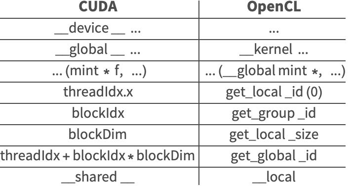
Since both CUDALink and OpenCLLink handle all the underlying bookkeeping for CUDA and OpenCL, the user need only concentrate on the kernel code. This section covers a CUDA-to-OpenCL translation. It is assumed that the user has used OpenCLLink to develop the function.
The following table summarizes some of the common changes in the kernel code needed to port OpenCL programs to CUDA.
This is a simple OpenCL function that takes input image and color negates it.
src = "
__kernel void imageColorNegate(__global mint * img, mint width, mint height, mint channels) {
    mint ii;
	int xIndex = get_global_id(0);
	int yIndex = get_global_id(1);
	int index = channels*(xIndex + yIndex*width);
	if (xIndex < width && yIndex < height) {
		for (ii = 0; ii < channels; ii++)
			img[index+ii] = 255 - img[index+ii];
    }
}
";
Recall that to launch the OpenCL function you perform the following.
Needs["OpenCLLink`"]
colorNegate = OpenCLFunctionLoad[src, "imageColorNegate", {{_Integer, _, "InputOutput"}, _Integer, _Integer, _Integer}, {16, 16}];
{height, width, channels} = ImageDimensions[[image]]~Join~{ImageChannels[[image]]};
colorNegate[[image], width, height, channels]
The following is changed in order to port to CUDA.
In many cases, the above are the only required changes for OpenCL-to-CUDA porting in the Wolfram Language. There are a handful of other one-to-one function translations that are readily accessible in an OpenCL or CUDA programming guide.
src = "
__global__ void imageColorNegate(mint * img, mint width, mint height, mint channels) {
    mint ii;
	int xIndex = threadIdx.x + blockIdx.x*blockDim.x;
	int yIndex = threadIdx.y + blockIdx.y*blockDim.y;
	int index = channels*(xIndex + yIndex*width);
	if (xIndex < width && yIndex < height) {
		for (ii = 0; ii < channels; ii++)
			img[index+ii] = 255 - img[index+ii];
    }
}
";
This is the exact Wolfram Language functions done for OpenCL, but replacing OpenCLFunctionLoad load with CUDAFunctionLoad.
Needs["CUDALink`"]
colorNegate = CUDAFunctionLoad[src, "imageColorNegate", {{_Integer, _, "InputOutput"}, _Integer, _Integer, _Integer}, {16, 16}];
{height, width, channels} = ImageDimensions[[image]]~Join~{ImageChannels[[image]]};
colorNegate[[image], width, height, channels]
An alternative to find and replace the mechanism shown above is to generate the kernel code symbolically and manipulate it in the Wolfram Language. The following section covers that approach.
Symbolic Code Generation
The Wolfram Language provides SymbolicC, which permits a hierarchical view of C code as the Wolfram Language's own. This makes it well suited to creating, manipulating, and optimizing C code.
In conjunction with this capability, users can generate CUDA kernel code for several different targets, allowing greater portability, less platform dependency, and better code optimization.
An advantage of using SymbolicC is that you can ensure that the C code contains no syntactical errors, you can generate CUDA programs using SymbolicC and run them using CUDAFunctionLoad, and you can ease the porting of CUDA to OpenCL (or vice versa).
This section uses CUDALink's symbolic code-generation capabilities to write an "RGB"-to-"HSV" and "RGB"-to-"HSB" color converter. This conversion is a fairly common operation for image and video processing.
For this tutorial, the CUDALink application must first be loaded.
Needs["CUDALink`"]Introduction
CUDALink includes symbolic tools that help in writing kernels using SymbolicC.
| SymbolicCUDAFunction | symbolic representation of a CUDA function |
| SymbolicCUDABlockIndex | symbolic representation of a block index CUDA call |
| SymbolicCUDAThreadIndex | symbolic representation of a thread index CUDA call |
| SymbolicCUDABlockDimension | symbolic representation of a block dimension CUDA call |
| SymbolicCUDACalculateKernelIndex | symbolic representation of a CUDA index calculation |
| SymbolicCUDADeclareIndexBlock | symbolic representation of a CUDA index declaration |
Symbolic representations of CUDA programs.
The following is an example kernel written symbolically.
symb = SymbolicCUDAFunction["kernelFunctionName", {{CPointerType["mint"], "arg1"}, {"mint", "arg2"}},
	CBlock[{
	SymbolicCUDADeclareIndexBlock[2],
	CIf[COperator[Less, {"index", "arg2"}],
	CAssign[CArray["arg1", "index"], 33]
	]
	}]
	]
This displays the C code generated using ToCCodeString.
ToCCodeString[symb]Another reason for writing code symbolically is that you can rewrite the above kernel to OpenCL form by just changing the "CUDA" instances to "OpenCL".
Needs["OpenCLLink`"]symb = SymbolicOpenCLFunction["kernelFunctionName", {{CPointerType["mint"], "arg1"}, {"mint", "arg2"}},
CBlock[{
SymbolicOpenCLDeclareIndexBlock[2],
CIf[COperator[Less, {"index", "arg2"}],
CAssign[CArray["arg1", "index"], 33]
]
}]
]Again, you display the C code using ToCCodeString.
ToCCodeString[symb]Simple Kernel
CUDALink provides utility functions that perform common GPU kernel programming tasks as discussed above. With them, you will write your first kernel function.
First, load the CUDALink application.
Needs["CUDALink`"]Your first function will take an integer array and set all its elements to 0. You first need to define your function prototype. The function will be called "firstKernel", accepting an input list and the list size. Use the utility functions as follows.
SymbolicCUDAFunction["firstKernel", {{CPointerType["mint"], "list"}, {"mint", "listSize"}}, CBlock[{
}]]//ToCCodeString
Since you will be building this example incremental, and to avoid writing the above each time, you can define a helper function for this example.
FirstKernel[api_, body___] := ToCCodeString[
If[api === "CUDA", SymbolicCUDAFunction, SymbolicOpenCLFunction]["firstKernel", {{CPointerType["mint"], "list"}, {"mint", "listSize"}}, CBlock[{
body
}]]]FirstKernel["CUDA"]Getting the Index
Using the SymbolicCUDADeclareIndexBlock, you can find the index of the list element based on the thread index, block index, and block dimensions.
FirstKernel["CUDA",
	SymbolicCUDADeclareIndexBlock[1]
	]
Declaring the Body
Since you can launch more threads than you actually have elements, you need to place the function body inside an "if" guard. Not doing so might make your program unpredictable.
FirstKernel["CUDA",
	SymbolicCUDADeclareIndexBlock[1],
	CIf[COperator[Less, {"index", "listSize"}], CBlock[{
	}]]
	]
You can now define the body of the kernel. The body is trivial, setting each element in the list to 0.
FirstKernel["CUDA",
	SymbolicCUDADeclareIndexBlock[1],
	CIf[COperator[Less, {"index", "listSize"}], CBlock[{
	CAssign[CArray["list", "index"], 0]
	}]]
	]
Testing the First Kernel
Import the CUDALink package, if you have not already done so.
Needs["CUDALink`"]listSize = 100;
list = ConstantArray[6, listSize];This generates the source code.
src = FirstKernel["CUDA",
	SymbolicCUDADeclareIndexBlock[1],
	CIf[COperator[Less, {"index", "listSize"}], CBlock[{
	CAssign[CArray["list", "index"], 0]
	}]]
]zero = CUDAFunctionLoad[src, "firstKernel", {{_Integer}, _Integer}, 16]zero[list, listSize]Advanced Kernels
In this section you are shown how to write an RGB-to-HSV and RGB-to-HSB converter. These are common conversions in image and video processing.
Helper Functions
SymbolicC only includes C constructs. To make your code more Wolfram Language-like, define the following.
CWhich[x_, y_] := CIf[x, y];
CWhich[x_, y_, tail__] :=
	CIf[x,
	{y},
	If[TrueQ[First[{tail}]],
	Rest[{tail}],
	CWhich[tail]
	]
	];
CWhich rewrites your expression using CIf.
CWhich[
	COperator[Equal, {x, 1}],
		CAssign[x, 4],
	COperator[Equal, {x, 4}],
		CAssign[x, 7],
	COperator[And, {COperator[Equal, {y, 6}], COperator[Unequal, {j, 5}]}],
		CAssign[x, 9],
	True,
		CAssign[x, 11]
	]
This converts the above expression into C code.
ToCCodeString[%]Use this to reimplement the code found in FileNameJoin[{$CUDALinkPath,"SupportFiles","colorConvert.cu"}].
Color Convert
Break up the problem into its components. First, define the RGB-to-Hue function. This function is common between RBG-to-HSV and RGB-to-HSB.
The following writes the RGB-to-H convert function.
RGB2H = {
	CWhich[
	COperator[Equal, {maxPixel, minPixel}], CAssign[x, 0],
	COperator[Equal, {maxPixel, r}], {
	CAssign[x, COperator[Plus, {COperator[Times, {60.0, COperator[Divide, {COperator[Subtract, {g, b}], COperator[Subtract, {maxPixel, minPixel}]}]}], 360.0}]],
	CIf[COperator[GreaterEqual, {x, 360.0}],
	CAssign[x, COperator[Subtract, {x, 360.0}]]
	]},
	COperator[Equal, {maxPixel, g}], CAssign[x, COperator[Plus, {COperator[Times, {60.0, COperator[Divide, {COperator[Subtract, {b, r}], COperator[Subtract, {maxPixel, minPixel}]}]}], 120.0}]],
	COperator[Equal, {maxPixel, b}], CAssign[x, COperator[Plus, {COperator[Times, {60.0, COperator[Divide, {COperator[Subtract, {r, g}], COperator[Subtract, {maxPixel, minPixel}]}]}], 240.0}]]],
	CAssign[x, COperator[Divide, {x, 360.0}]]
	};
This transforms the expression into C.
ToCCodeString[RGB2H, "Indent" -> Automatic]This writes the saturation in case of HSB.
ToCCodeString[RGB2HSBS = CIf[COperator[Equal, {maxPixel, 0}],
	CAssign[y, 0],
	CAssign[y, COperator[Divide, {COperator[Subtract, {maxPixel, minPixel}], maxPixel}]]], "Indent" -> Automatic]
This defines the formula to find the brightness.
RGB2HSBB = CAssign[z, COperator[Times, {0.5, COperator[Plus, {maxPixel, minPixel}]}]]ToCCodeString[RGB2HSVS = CIf[COperator[Equal, {maxPixel, minPixel}],
CAssign[y, 0],
{CIf[COperator[GreaterEqual, {COperator[Plus, {maxPixel, minPixel}], 1}],
CAssign[y, COperator[Divide, {COperator[Subtract, {maxPixel, minPixel}], COperator[Plus, {maxPixel, minPixel}]}]],
CAssign[y, COperator[Divide, {COperator[Subtract, {maxPixel, minPixel}], COperator[Plus, {-1, maxPixel, minPixel}]}]]]}], "Indent" -> Automatic]RGB2HSVV = CAssign[z, maxPixel]Notice that you need to define what max and min are.
CMax[x_, y_] := CCall[max, {x, y}]CMax[{x_, y_, tail___}] := CMax[x, CMax[y, tail]]CMin[x_, y_] := CCall[min, {x, y}]CMin[{x_, y_, tail___}] := CMin[x, CMin[y, tail]]Putting everything together, RGB2HSV is defined as follows.
ToCCodeString[RGB2HSV = {
	CAssign[maxPixel, CMax[{r, g, b}]],
	CAssign[minPixel, CMin[{r, g, b}]],
	RGB2H,
	RGB2HSVS,
	RGB2HSVV
	}, "Indent" -> Automatic]
Similarly, RGB2HSB is defined as follows.
ToCCodeString[RGB2HSB = {
	CAssign[maxPixel, CMax[{r, g, b}]],
	CAssign[minPixel, CMin[{r, g, b}]],
	RGB2H,
	RGB2HSBS,
	RGB2HSBB
	}, "Indent" -> Automatic]
To generate the kernel function, you use the Wolfram Language's functional capabilities. This defines a helper function.
ToGPUKernelFunction[funName_, fun_, targetPrecision_] :=
	With[{realType = If[targetPrecision === "Single", "float", "double"]}, SymbolicCUDAFunction[funName, {{CPointerType[realType], "input"}, {CPointerType[realType], "output"}, {"mint", "width"}, {"mint", "height"}}, CBlock[{
	SymbolicCUDADeclareIndexBlock[2, "width"],
	CAssign[TimesBy, "index", 3],
	CDeclare[realType, {x, y, z, maxPixel, minPixel}],
	CIf[COperator[And, {COperator[Less, {"xIndex", "width"}], COperator[Less, {"yIndex", "height"}]}], {
	MapThread[CDeclare[realType, CAssign[#1, CArray["input", COperator[Plus, {"index", #2}]]]]&, {{"r", "g", "b"}, {0, 1, 2}}],
	fun,
	MapThread[CAssign[CArray["output", COperator[Plus, {"index", #1}]], #2]&, {{0, 1, 2}, {"x", "y", "z"}}]
	}]
	}]]
	]
Using the above function, you can define the RGB-to-HSB operation to use single-precision arithmetic.
ToCCodeString[ToGPUKernelFunction["rgb2hsb", RGB2HSB, "Single"], "Indent" -> Automatic]This generates the code for double precision.
ToCCodeString[ToGPUKernelFunction["rgb2hsb", RGB2HSB, "Double"], "Indent" -> Automatic]The same can be done for the RGB-to-HSV operation.
ToCCodeString[ToGPUKernelFunction["rgb2hsv", RGB2HSV, "Single"], "Indent" -> Automatic]Running the Program
The above code can be run using CUDAFunctionLoad. First, generate the source in single precision.
src = ToCCodeString[ToGPUKernelFunction["rgb2hsb", RGB2HSB, "Single"]];Before running the code on the GPU, you need to define some parameters that are required. This defines the input and output image. Notice that the output is of type Real, since HSV and HSB are real valued.
img = [image];
InputImage = ImageData[img];
OutputImage = ConstantArray[1.0, Dimensions[InputImage]];
{height, width} = ImageDimensions[img];
This loads the function into the Wolfram Language.
rgb2hsb = CUDAFunctionLoad[src, "rgb2hsb", {{"Float", "Input"}, {"Float", "Output"}, _Integer, _Integer}, {16, 16}]res = rgb2hsb[InputImage, OutputImage, width, height];Image[First[res], ColorSpace -> "HSB"]