Delay Differential Equations
| Comparison and Contrast with ODEs | The Method of Steps |
| Propagation and Smoothing of Discontinuities | Examples |
| Storing History Data |
A delay differential equation is a differential equation where the time derivatives at the current time depend on the solution and possibly its derivatives at previous times:
Instead of a simple initial condition, an initial history function ![]() needs to be specified. The quantities
needs to be specified. The quantities ![]() and
and ![]() are called the delays or time lags. The delays may be constants, functions
are called the delays or time lags. The delays may be constants, functions ![]() and
and ![]() of
of ![]() (time-dependent delays), or functions
(time-dependent delays), or functions ![]() and
and ![]() (state-dependent delays). Delay equations with delays
(state-dependent delays). Delay equations with delays ![]() of the derivatives are referred to as neutral delay differential equations (NDDEs).
of the derivatives are referred to as neutral delay differential equations (NDDEs).
The equation processing code in NDSolve has been designed so that you can input a delay differential equation in essentially mathematical notation.
| x[t-τ] | dependent variable x with delay τ |
| x[t /; t≤t0]ϕ | specification of initial history function as expression ϕ for t less than t0 |
Inputting delays and initial history.
Currently, the implementation for DDEs in NDSolve only supports constant delays.
sol = NDSolve[{x''[t] + x[t - 1] == 0, x[t /; t ≤ 0] == t ^ 2}, x, {t, -1, 5}]Plot[Evaluate[{x[t], x'[t], x''[t]} /. First[sol]], {t, -1, 5}, PlotRange -> All]For simplicity, this documentation is written assuming that integration always proceeds from smaller to larger ![]() . However, NDSolve supports integration in the other direction if the initial history function is given for values above
. However, NDSolve supports integration in the other direction if the initial history function is given for values above ![]() and the delays are negative.
and the delays are negative.
nsol = NDSolve[{x''[t] + x[t + 1] == 0, x[t /; t ≥   0] == t ^ 2}, x, {t, -5, 1}];
Plot[Evaluate[{x[t], x'[t], x''[t]} /. First[nsol]], {t, -5, 1}, PlotRange -> All]
Comparison and Contrast with ODEs
While DDEs look a lot like ODEs the theory for them is quite a bit more complicated and there are some surprising differences from ODEs. This section will show a few examples of the differences.
Manipulate[
	Module[{sol = NDSolve[{x'[t] == x[t - 1](1 - x[t]), x[t /; t ≤ 0] == ϕ}, x, {t, -2, 2}]},
	Plot[Evaluate[x[t] /. First[sol]], {t, -2, 2}]], {ϕ, {Exp[t], Cos[t], 1 - t, 1 - Sin[t]}}]
As long as the initial function satisfies ![]() , the solution for
, the solution for ![]() is always 1. [Z06] With ODEs, you could always integrate backward in time from a solution to obtain the initial condition.
is always 1. [Z06] With ODEs, you could always integrate backward in time from a solution to obtain the initial condition.
Manipulate[
	Module[{T = 50, sol, x, t}, sol = First[x /. NDSolve[{x'[t] == a x[t](1 - x[t - 1]), x[t /; t ≤ 0] == 0.1}, x, {t, 0, T}]];
	If[pp, ParametricPlot[{sol[t], sol[t - 1]}, {t, 1, T}, PlotRange -> {{0, 3}, {0, 3}}],
	Plot[sol[t], {t, 0, T}, PlotRange -> {{0, 50}, {0, 3}}]]], {{pp, False, "Plot in Phase Plane"}, {False, True}}, {{a, 1}, 0, 2}]
For ![]() , the solutions are monotonic, for
, the solutions are monotonic, for ![]() the solutions oscillate, and for
the solutions oscillate, and for ![]() the solutions approach a limit cycle. Of course, for the scalar ODE, solutions are monotonic independent of
the solutions approach a limit cycle. Of course, for the scalar ODE, solutions are monotonic independent of ![]() .
.
sol1 = First[NDSolve[{x'[t] == Sin[x[t - 20]], x[t /; t ≤ 0] == .0001}, x, {t, 0, 500}]];
sol2 = First[NDSolve[{x'[t] == Sin[x[t - 20]], x[t /; t ≤ 0] == .00011}, x, {t, 0, 500}]];Plot[Evaluate[x[t] /. {sol1, sol2}], {t, 0, 500}]This simple scalar delay differential equation has chaotic solutions and the motion shown above looks very much like Brownian motion. [S07] As the delay ![]() is increased beyond
is increased beyond ![]() a limit cycle appears, followed eventually by a period-doubling cascade leading to chaos before
a limit cycle appears, followed eventually by a period-doubling cascade leading to chaos before ![]() .
.
Grid[Table[sol = First[NDSolve[{x'[t] == Sin[x[t - τ]], x[t /; t ≤ 0] == .1}, x, {t, 100τ, 200τ}, MaxSteps -> Infinity]];
	{ParametricPlot[Evaluate[{x[t - 1], x[t]} /. sol], {t, 101τ, 200τ}].
	Plot[Evaluate[x[t] /. sol], {t, 100τ, 200τ}]}, {τ, 4.9, 5.1, .1}]]
Stability is much more complicated for delay equations as well. It is well known that the linear ODE test equation ![]() has asymptotically stable solutions if
has asymptotically stable solutions if ![]() and is unstable if
and is unstable if ![]() .
.
The closest corresponding DDE is ![]() . Even if you consider just real
. Even if you consider just real ![]() and
and ![]() the situation is no longer so clear-cut. Shown below are some plots of solutions indicating this.
the situation is no longer so clear-cut. Shown below are some plots of solutions indicating this.
Block[{λ = 1 / 2, μ = -1, T = 25}, Plot[Evaluate[First[x[t] /. NDSolve[{x'[t] == λ x[t] + μ x[t - 1], x[t /; t ≤ 0] == 1 - t}, x, {t, 0, T}]]], {t, 0, T}, PlotRange -> All]]Block[{λ = -7 / 2, μ = 4, T = 25}, Plot[Evaluate[First[x[t] /. NDSolve[{x'[t] == λ x[t] + μ x[t - 1], x[t /; t ≤ 0] == 1 - t}, x, {t, 0, T}]]], {t, 0, T}, PlotRange -> All]]So the solution can be stable with ![]() and unstable with
and unstable with ![]() depending on the value of
depending on the value of ![]() . A Manipulate is set up below so that you can investigate the
. A Manipulate is set up below so that you can investigate the ![]() plane.
plane.
Manipulate[Module[{T = 25, x, t}, Plot[Evaluate[First[x[t] /. NDSolve[{x'[t] == λ x[t] + μ x[t - 1], x[t /; t ≤ 0] == 1 - t}, x, {t, 0, T}]]], {t, 0, T}, PlotRange -> All]], {λ, -5, 5}, {μ, -5, 5}]Propagation and Smoothing of Discontinuities
The way discontinuities are propagated by the delays is an important feature of DDEs and has a profound effect on numerical methods for solving them.
sol = First[NDSolve[{x'[t] == x[t - 1], x[t /; t ≤ 0] == 1}, x, {t, -1, 3}]]Plot[Evaluate[{x[t], x'[t], x''[t]} /. sol], {t, -1, 3}]In the example above, ![]() is continuous, but there is a jump discontinuity in
is continuous, but there is a jump discontinuity in ![]() at
at ![]() since approaching from the left the value is
since approaching from the left the value is ![]() , given by the derivative of the initial history function
, given by the derivative of the initial history function ![]() , while approaching from the right the value is given by the DDE, giving
, while approaching from the right the value is given by the DDE, giving ![]() .
.
Near ![]() , we have by the continuity of
, we have by the continuity of ![]() at
at ![]()
![]() and so
and so ![]() is continuous at
is continuous at ![]() .
.
Differentiating the equation, we can conclude that ![]() so
so ![]() has a jump discontinuity at
has a jump discontinuity at ![]() . Using essentially the same argument as above, we can conclude that at
. Using essentially the same argument as above, we can conclude that at ![]() the second derivative is continuous.
the second derivative is continuous.
Similarly, ![]() is continuous at
is continuous at ![]() or, in other words, at
or, in other words, at ![]() ,
, ![]() is
is ![]() times differentiable. This is referred to as smoothing and holds generally for non-neutral delay equations. In some cases the smoothing can be faster than one order per interval.[Z06]
times differentiable. This is referred to as smoothing and holds generally for non-neutral delay equations. In some cases the smoothing can be faster than one order per interval.[Z06]
For neutral delay equations the situation is quite different.
sol = First[NDSolve[{x'[t] == -x'[t - 1], x[t /; t ≤ 0] == t}, x, {t, -1, 3}]]Plot[Evaluate[{x[t], x'[t]} /. sol], {t, -1, 3}]It is easy to see that the solution is piecewise with ![]() continuous. However,
continuous. However,
which has a discontinuity at every non-negative integer.
In general, there is no smoothing of discontinuities for neutral DDEs.
The propagation of discontinuities is very important from the standpoint of numerical solvers. If the possible discontinuity points are ignored, then the order of the solver will be reduced. If a discontinuity point is known, a more accurate solution can be found by integrating just up to the discontinuity point and then restarting the method just past the point with the new function values. This way, the integration method is used on smooth parts of the solution, leading to better accuracy and fewer rejected steps. From any given discontinuity points, future discontinuity points can be determined from the delays and detected by treating them as events to be located.
When there are multiple delays, the propagation of discontinuities can become quite complicated.
sol = NDSolve[{x'[t] == x[t](x[t - Pi] - x'[t - 1]), x[t /; t ≤ 0] == Cos[t]}, x, {t, -1, 8}]Plot[Evaluate[{x[t], x'[t]} /. First[sol]], {t, -1, 8}, PlotRange -> All]It is clear from the plot that there is a discontinuity at each non-negative integer as would be expected from the neutral delay ![]() . However, looking at the second and third derivative, it is clear that there are also discontinuities associated with points like
. However, looking at the second and third derivative, it is clear that there are also discontinuities associated with points like ![]() ,
, ![]() ,
, ![]() propagated from the jump discontinuities in
propagated from the jump discontinuities in ![]() .
.
Plot[Evaluate[x''[t] /. First[sol]], {t, 2.5, 5.5}, PlotRange -> {-3, 3}]In fact, there is a whole tree of discontinuities that are propagated forward in time. A way of determining and displaying the discontinuity tree for a solution interval is shown in the subsection below.
Discontinuity Tree
DiscontinuityTree[t0_,   Tend_, delays_]  :=
	Module[{dt, next, ord},
	ord[t_] := Infinity;
	ord[t0] = 0;
	next[b_, order_, del_] := Map[dt[b, #, order, del]&, del];
	dt[t_, {d_, nq_}, order_, del_]  := Module[{b = t + d},
	If[b ≤ Tend,
	o   = order + Boole[!nq];
	ord[b] = Min[ord[b], o];
	Sow[{t -> b, d}];
	next[b, o, del]]];
	rules = Reap[next[t0, 0, delays]][[2, 1]];
	rules = Tally[rules][[All, 1]];
	f[x_ ? NumericQ] := {x, ord[x]};
	f[a_ -> b_] := f[a] -> f[b];
	rules[[All, 1]] = Map[f, rules[[All, 1]]];
rules]tree = Tally[DiscontinuityTree[0, 8, {{1, True}, {π, False}}]][[All, 1]]ShowDiscontinuity[{dt_, o_}, ifun_, Δ_] :=
Quiet[
Plot[Evaluate[{Derivative[o][ifun][t], Derivative[o + 1][ifun][t]}], {t, dt - Δ, dt + Δ}, Exclusions -> {dt}, ExclusionsStyle -> Red, Frame -> True, FrameLabel -> {None, None, {Derivative[o][x][t], Derivative[o + 1][x][t]}, None}]]LayeredGraphPlot[tree, Left, VertexSize -> .3, VertexShapeFunction -> Function[Tooltip[{White, Disk[#, .25], Black, Text[#2[[1]], #1]}, ShowDiscontinuity[#2, First[x /. sol], 1]]]]Storing History Data
Once the solution has advanced beyond the first discontinuity point, some of the delayed values that need to be computed are outside the domain of the initial history function, and the computed solution needs to be used to get the values, typically by interpolating between steps previously taken. For the DDE solution to be accurate it is essential that the interpolation be as accurate as the method. This is achieved by using dense output for the ODE integration method (the output you get if you use the option InterpolationOrder->All in NDSolve). NDSolve has a general algorithm for obtaining dense output from most methods, so you can use just about any method as the integrator. Some methods, including the default for DDEs, have their own way of getting dense output, which is usually more efficient than the general method. Methods that are low enough order, such as "ExplicitRungeKutta" with "DifferenceOrder"->3 can just use a cubic Hermite polynomial as the dense output, so there is essentially no extra cost in keeping the history.
Since the history data is accessed frequently, it needs to have a quick lookup mechanism to determine which step to interpolate within. In NDSolve, this is done with a binary search mechanism and the search time is negligible compared with the cost of actual function evaluation.
The data for each successful step is saved before attempting the next step, and is saved in a data structure that can repeatedly be expanded efficiently. When NDSolve produces the solution, it simply takes this data and restructures it into an InterpolatingFunction object, so DDE solutions are always returned with dense output.
The Method of Steps
For constant delays, it is possible to get the entire set of discontinuities as fixed time. The idea of the method of steps is to simply integrate the smooth function over these intervals and restart on the next interval, being sure to reevaluate the function from the right. As long as the intervals do not get too small, the method works quite well in practice.
The method currently implemented for NDSolve is based on the method of steps.
Symbolic Method of Steps
This section defines a symbolic method of steps that illustrates how the method works. Note that to keep the code simpler and more to the point, it does not do any real argument checking. Also, the data structure and lookup for the history is not done in an efficient way, but for symbolic solutions this is a minor issue.
IntegrateSmooth[rhs_, history_, delayvars_, pfun_, dvars_, {t_, t0_, t1_}] := Module[{dvt, tau, hrule, dvrule, dvrules, oderhs, ode, init, sol},
	dvt[tau_] = Map[#[tau]&, dvars];
	hrule[pos_] := Thread[dvars -> Map[Function[Evaluate[{t}], #]&, history[[pos]]]];
	dvrule[(dv_)[z_]] := Module[{delay, pos},
	delay = t - z;
	pos = pfun[t0 - delay];
	dv[z] -> (dv[z] /. hrule[pos])];
	dvrules = Map[dvrule, delayvars];
	oderhs = rhs /. dvrules;
	ode = Thread[D[dvt[t], t] == oderhs];
	init  = Thread[dvt[t0] == (dvt[t0]  /. hrule[-1])];
	sol = DSolve[{ode, init}, dvars, t];
	If[Head[sol] === DSolve || Length[sol] == 0,
	Message[DDESteps::stuck, ode, init];
	Throw[$Failed]];
	dvt[t] /. First[sol]
	];
DDESteps::stuck = "DSolve was not able to find a solution for `1` with initial conditions `2`.";DDESteps[rhsin_, phin_, dvarsin_, {t_, tinit_, tend_}] := Module[{rhs = Listify[rhsin], phi = Listify[phin], dvars = Listify[dvarsin], history, delayvars, delays, dtree, intervals, p, pfun, next, pieces, hfuns},
history = {phi};
delayvars = Cases[rhs, (v : ((dv_[z_] | Derivative[1][dv_][z_]) /; (MemberQ[dvars, dv] && UnsameQ[z, t]))) -> {v, t - z}, Infinity];
{delayvars, delays} = Map[Union, Transpose[delayvars]];
dtree = DiscontinuityTree[tinit, tend, Map[{#, True}&, delays]];
dtree = Union[Flatten[{tinit, tend, dtree[[All, 1, 2, 1]]}]];
dtree = SortBy[dtree, N];
intervals = Partition[dtree, 2, 1];
p = 2;
pfun = Join[{{1, t < tinit}}, Apply[Function[{p++, #1 ≤ t < #2}], intervals, {1}]];
pfun = Function[Evaluate[{t}], Evaluate[Piecewise[pfun, p]]];
Catch[Do[
next = IntegrateSmooth[rhs, history, delayvars, pfun, dvars, Prepend[interval, t]];
history = Append[history, next],
{interval, intervals}]];
pieces = Flatten[{t < tinit, Apply[(#1 ≤ t < #2)&, Drop[intervals, -1], {1}], Apply[(#1 ≤ t ≤ #2)&, Last[intervals]]}];
pieces = Take[pieces, Length[history]];
hfuns = Map[Function[Evaluate[{t}], Evaluate[Piecewise[Transpose[{#, pieces}], Indeterminate]]]&, Transpose[history]];
Thread[dvars -> hfuns]
];
Listify[x_List] := x;
Listify[x_] := {x};sol = DDESteps[x[t - 1] - x[t], Sin[t], x, {t, 0, 3}]Plot[Evaluate[{x[t], x'[t]} /. sol], {t, 0, 3}]ndsol = First[NDSolve[{x'[t] == -x[t] + x[t - 1], x[t /; t ≤ 0] == Sin[t]}, x, {t, 0, 3}]];
Plot[Evaluate[(x[t] /. sol) - (x[t] /. ndsol)], {t, 0, 3}, PlotRange -> All]The method will also work for neutral DDEs.
sol = DDESteps[x'[t - 1] - x[t], Sin[t], x, {t, 0, 3}]Plot[Evaluate[{x[t], x'[t]} /. sol], {t, 0, 3}]ndsol = First[NDSolve[{x'[t] == -x[t] + x'[t - 1], x[t /; t ≤ 0] == Sin[t]}, x, {t, 0, 3}]];
Plot[Evaluate[(x[t] /. sol) - (x[t] /. ndsol)], {t, 0, 3}, PlotRange -> All]The symbolic method will also work with symbolic parameter values as long as DSolve is still able to find the solution.
sol = DDESteps[λ x[t] + μ x[t - 1], t, x, {t, 0, 2}]The reason the code was designed to take lists was so that it would work with systems.
ssol = DDESteps[{y[t], -x[t - 1]}, {t ^ 2, 2 t}, {x, y}, {t, 0, 5}]Plot[Evaluate[{x[t], y[t]} /. ssol], {t, 0, 5}]ndssol = First[NDSolve[{x'[t] == y[t], y'[t] == -x[t - 1], x[t /; t ≤ 0] == t ^ 2, y[t /; t ≤ 0] == 2 t}, {x, y}, {t, 0, 5}]];
Plot[Evaluate[({x[t], y[t]} /. ssol) - ({x[t], y[t]} /. ndssol)], {t, 0, 5}]Since the method computes the discontinuity tree, it will also work for multiple constant delays. However, with multiple delays, the solution may become quite complicated quickly and DSolve can bog down with huge expressions.
sol = DDESteps[x[t](x[t - Log[2]] - x'[t - 1]), 1, x, {t, 0, 2}]Plot[Evaluate[{x[t], x'[t]} /. sol], {t, 0, 2}]ndsol = First[NDSolve[{x'[t] == x[t](x[t - Log[2]] - x'[t - 1]), x[t /; t ≤ 0] == 1}, x, {t, 0, 2}]];
Plot[Evaluate[(x[t] /. sol) - (x[t] /. ndsol)], {t, 0, 2}, PlotRange -> All]Examples
Lotka–Volterra Equations with Delay
The Lotka–Volterra system models the growth and interaction of animal species assuming that the effect of one species on another is continuous and immediate. A delayed effect of one species on another can be modeled by introducing time lags in the interaction terms.
With no delays, ![]() and the system (1) has an invariant
and the system (1) has an invariant ![]() that is constant for all
that is constant for all ![]() and there is a (neutrally) stable periodic solution.
and there is a (neutrally) stable periodic solution.
lvsystem[τ1_, τ2_] := {
	Subscript[Y, 1]'[t] == Subscript[Y, 1][t](Subscript[Y, 2][t - τ1] - 1), Subscript[Y, 1][0] == 1,
	Subscript[Y, 2]'[t] == Subscript[Y, 2][t](2 - Subscript[Y, 1][t - τ2]), Subscript[Y, 2][0] == 1};
lv = First[NDSolve[lvsystem[0, 0], {Subscript[Y, 1], Subscript[Y, 2]}, {t, 0, 25}]];
lvd = Quiet[First[NDSolve[lvsystem[.01, 0], {Subscript[Y, 1], Subscript[Y, 2]}, {t, 0, 25}]]];
ParametricPlot[Evaluate[{Subscript[Y, 1][t], Subscript[Y, 2][t]} /. {lv, lvd}], {t, 0, 25}]
In this example, the effect of even a small delay is to destabilize the periodic orbit. With different parameters in the delayed Lotka–Volterra system it has been shown that there are globally attractive equilibria.[TZ08]
Enzyme Kinetics
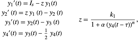
modeling enzyme kinetics where ![]() is a substrate supply maintained at a constant level and
is a substrate supply maintained at a constant level and ![]() molecules of the end product
molecules of the end product ![]() inhibits the reaction step
inhibits the reaction step ![]() . [HNW93]
. [HNW93]
The system has an equilibrium when ![]() ,
, ![]() , and
, and ![]() .
.
Manipulate[
	Module[{t, y1, y2, y3, y4, z, sol},
	z = k1 / (1 + α y4[t - τ] ^ n);
	sol = First[NDSolve[{
	y1'[t] == Is - z y1[t], y1[t /; t ≤ 0] == Is * (1 + α (2 Is) ^ n) + ϵ,
	y2'[t] == z y1[t] - y2[t], y2[t /; t ≤ 0]   == Is,
	y3'[t]  ==   y2[t] - y3[t], y3[t /; t ≤ 0]   == Is,
	y4'[t] == y3[t] - y4[t] / 2, y4[t /; t ≤ 0]   == 2Is},
	{y1, y2, y3, y4}, {t, 0, 200}]];
Plot[Evaluate[{y1[t], y2[t], y3[t], y4[t]} /. sol], {t, 0, 200}]], {{Is, 10.5}, 1, 20}, {{α, 0.0005}, 0, .001}, {{k1, 1}, 0, 2}, {{n, 3}, 1, 10, 1}, {{τ, 4}, 0, 10}, {{ϵ, 0.1}, 0, .25}]Mackey–Glass Equation
The Mackey–Glass equation ![]() was proposed to model the production of white blood cells. There are both periodic and chaotic solutions.
was proposed to model the production of white blood cells. There are both periodic and chaotic solutions.
sol = First[ NDSolve[{x'[t] == (1 / 4) x[t - 15] / (1 + x[t - 15] ^ 10) - x[t] / 10, x[t /; t ≤ 0] == 1 / 2}, x, {t, 0, 500}]];
ParametricPlot[Evaluate[{x[t], x[t - 15]} /. sol], {t, 300, 500}]sol = First[ NDSolve[{x'[t] == (1 / 4) x[t - 17] / (1 + x[t - 17] ^ 10) - x[t] / 10, x[t /; t ≤ 0] == 1 / 2}, x, {t, 0, 500}]];
ParametricPlot[Evaluate[{x[t], x[t - 17]} /. sol], {t, 300, 500}]sol = First[ NDSolve[{x'[t] == (1 / 4) x[t - 17] / (1 + x[t - 17] ^ 10) - x[t] / 10, x[t /; t ≤ 0] == 1 / 2}, x, {t, 0, 5000}, MaxSteps -> ∞]];
ParametricPlot3D[Evaluate[{x[t], x[t - 17], x[t - 34]} /. sol], {t, 500, 5000}]It is interesting to check the accuracy of the chaotic solution.
solrk = First[ NDSolve[{x'[t] == (1 / 4) x[t - 17] / (1 + x[t - 17] ^ 10) - x[t] / 10, x[t /; t ≤ 0] == 1 / 2}, x, {t, 0, 5000}, MaxSteps -> ∞, Method -> {"ExplicitRungeKutta", "DifferenceOrder" -> 3}]];
ListPlot[Table[{t, RealExponent[(x[t] /. sol) - (x[t] /. solrk)]}, {t, 17, 5000, 17}]]
By the end of the interval, the differences between methods is order 1. Large deviation is typical in chaotic systems and in practice it is not possible or even necessary to get a very accurate solution for a large interval. However, if you do want a high quality solution, NDSolve allows you to use higher precision. For DDEs with higher precision, the "StiffnessSwitching" method is recommended.
hpsol = First[ NDSolve[{x'[t] == (1 / 4) x[t - 17] / (1 + x[t - 17] ^ 10) - x[t] / 10, x[t /; t ≤ 0] == 1 / 2}, x, {t, 0, 5000}, MaxSteps -> ∞, Method -> "StiffnessSwitching", WorkingPrecision -> 32 ]];Plot[Evaluate[x[t] /. {hpsol, sol, solrk}], {t, 4900, 5000}, PlotRange -> All]