|
Chapter 4
Fitting Data to Linear Models
by Least-Squares Techniques
One of the most used functions of Experimental Data Analyst (EDA) is fitting data to linear models, especially straight lines and curves. This chapter discusses doing these types of fits using the most common technique: least-squares minimization.
The next section provides background information on this topic. Although it uses some functions from EDA for illustration, the purpose of the section is not to be an introduction to those functions; rather, this section is intended as an introduction to the issues in linear fitting that the EDA functions implement.
Subsequent sections of this chapter introduce and discuss the EDA functions that do least-squares linear fits.
4.1 Background Discussion
4.1.1 Linear Fits
This chapter discusses one of the most used functions of EDA: fitting data to linear models. Calling the dependent variable y and the independent one x, a general representation of such a model can be given.
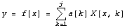
Here the a[k] are the parameters to be fit, and X[x, k] are called the "basis" functions.
As we shall see, the whole topic of fitting data to models is often surprisingly subtle.
By far the most common choice of basis functions are polynomials. Imagine we are trying to fit y versus x to a straight line.
y = a[0] + a[1] x
We are trying to determine a[0] and a[1], and the two basis functions are 1 and x.
Imagine we are fitting the data to a second-order polynomial.
y = a[0] + a[1] x + a[2] x^2
Now we are trying to fit to a[0], a[1], and a[2], and the basis functions are 1, x, and  . .
The use of the word "linear" is sometimes confusing in the context of fitting. It means that the model being fit is linear in the parameters to which we are fitting (i.e., the a[1] in the notation just introduced).
There is no such constraint on the basis functions. For example, we can fit y versus x data to trigonometric functions.
y = a[0] + a[1] Sin[2 x] + a[2] Sin[ 4 x] x] + a[2] Sin[ 4 x]
This is a linear fit, so the techniques discussed in this chapter may be used. The fact that the basis functions are not linear has no relevance in this context.
Now suppose we are fitting to an exponential function.
y = a[1] Exp[ -a[2]*x]
This is not a linear fit, since the parameter a[2] is nonlinear. Note that, in this example, the relationship can be made linear by transforming.
Writing aprime[1] = Log[a[1]] makes the relation a bit clearer.
Log[y] = aprime[1] - a[2]*x
Thus, fitting the logarithm of y versus x to a straight line effectively fits to the original equation and is linear. A small point about this sort of transformation is that it introduces biases into the parameters but often those biases can be ignored; this topic is discussed is Section 8.2.2.
Finally, imagine we are fitting to a more complex exponential.
y = a[1] Exp[ -a[2]*x] + a[3]*x
There is no simple transformation that will linearize this form. The techniques discussed in Chapter 5 on nonlinear techniques are required.
4.1.2 Least-Squares Techniques
The standard technique for performing linear fitting is by least-squares regression. This chapter discusses programs that use that algorithm.
However, as Emerson and Hoaglin point out, the technique is not without problems.
Various methods have been developed for fitting a straight line of the form:
y = a + bx
to the data
 , i = 1,..., n. , i = 1,..., n.
The best-known and most widely used method is least-squares regression, which involves algebraically simple calculations, fits neatly into the framework of inference built on the Gaussian distribution, and requires only a straightforward mathematical derivation. Unfortunately, the least-squares regression line offers no resistance. A wild data point can easily seize control of the fitted line and cause it to give a totally misleading summary of the relationship between y and x .
Reference: John D. Emerson and David C. Hoaglin, "Resistant Lines for y versus x," in David C. Hoaglin, Frederic Mosteller, and John W. Tukey, Understanding Robust and Exploratory Data Analysis (John Wiley, 1983, ISBN: 0-471-09777-2), pg. 129.
The central idea of the algorithm is that we are seeking a function f[x] which comes as close as possible to the actual experimental data. We let the data consist of N {x, y} pairs.
data = { {x[[1]],y[[1]]}, {x[[2]],y[[2]]},
... , {x[[N]],y[[N]]} }
Then for each data point the residual is defined as the difference between the experimental value of y and the value of y given by the function f evaluated at the corresponding value of x.
residual[[i]] = y[[i]] - f[ x[[i]] ]
First, we define the sum of the squares of the residuals.
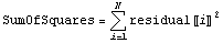
Then the least-squares technique minimizes the value of SumOfSquares.
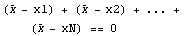
Here is a simple example. Imagine we have a succession of x values, which is the result of repeated measurements.
{x1, x2, ... , xN}
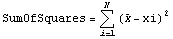
We wish to find an estimate of the expected value of x from this data. Call that estimate value  . Then, symbolically, we may write the sum of the squares. . Then, symbolically, we may write the sum of the squares.
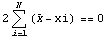
For this to be a minimum, the derivative with respect to  must be equal to zero. must be equal to zero.

We write out the sum.
We solve for  . .

But this is just the mean (i.e., average) of the xi. The mean has no resistance and a single contaminated data point can affect the mean to an arbitrary degree. For example, if x1 -> infinity, then so does  . It is in exactly this sense that the least-squares technique in general offers no resistance. . It is in exactly this sense that the least-squares technique in general offers no resistance.
Nonetheless, although EDA supplies functions that are resistant, the least-squares fitters discussed here are usually the first ones to try.
Usually we are fitting data to a model for which there is more than one parameter.
y = a[0] X[x,0] + a[1] X[x,1] + ... +
a[m] X[x,m]
The least-squares technique then takes the derivative of the sum of the squares of the residuals with respect to each of the parameters to which we are fitting and sets each to zero.
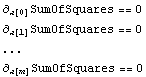
The analytic solution to this set of equations, then, is the result of the fit.
If the fit were perfect, then the resulting value of SumOfSquares would be exactly zero. The larger the value of SumOfSquares the less well the model fits the actual data.
4.1.3 Fitting to Data with Experimental Errors
As discussed in Chapter 3, in an experimental context in the physical sciences almost all measured quantities have an error because a perfect experimental apparatus does not exist. Chapter 3 also provides some guidelines for determining what are the values of those errors.
Nonetheless, all too often real experimental data in the sciences and engineering do not have explicit errors associated with the values of the dependent or independent variables. In this case the least-squares fitting techniques discussed in the previous subsection are usually used. As we shall see, EDA also provides extensions to this standard method with some reweighting heuristics.
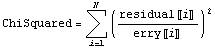
If there are assigned errors in the experimental data, say erry, then these errors are used to weight each term in the sum of the squares. If the errors are estimates of the standard deviation, such a weighted sum is called the "chi squared",  , of the fit. , of the fit.
The least-squares technique takes the derivatives of ChiSquared with respect to the parameters of the fit, sets each equation to zero, and solves the resulting set of equations. Thus, the only difference between this situation and the one discussed in the previous section is that we weight each residual with the inverse of the error.
Some references refer to the weights w[[i]] of a fit, while others call the errors erry the standard deviations.
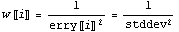
Also, some people refer to the "variance", which is the error or standard deviation squared.
If the data has errors in both the independent variable and the dependent one, say errx and erry, respectively, the fitting programs in EDA use what is called an "effective variance technique". For example, imagine we are fitting data to a[2] , and we have a data point where x = 3 +/- 0.1. , and we have a data point where x = 3 +/- 0.1.
In[1]:=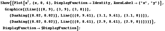
To a good approximation, the uncertainty in y, because of the errors in x, is the error in x times the slope of the line.
Thus, if we can assume that the errors in x are independent of the errors in y, we can combine erry and this term in quadrature to get an effective error in y.
Using these errors instead of erry is called the "effective variance technique." In general, if we are modeling
y = f[x]
then the algorithm involves replacing erry with
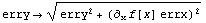
The square of the error erry is the "effective variance".
Notice that since this effective variance contains at least some of the values of the parameters to which we are fitting, the chi-squared is nonlinear in these parameters. This implies that a nonlinear fitting technique is, in principle, required. However, when the errors are small the nonlinearities are also small and almost always LinearFit can successfully iterate to a reasonable solution.
There are also some subtleties about the value of the independent variable to use in evaluating the derivatives of the function. In almost all cases, differences in fitted values using different ways of doing the evaluation are small compared to the errors in those values. Thus, LinearFit just evaluates the derivatives at the observed values of the independent variable.
When the fit is to a straight line, a particularly effective way to apply the effective variance technique is an algorithm called Brent minimization. This is the default for LinearFit. Section 4.4.1.2 discusses this further.
4.1.4 Evaluating the Goodness of a Fit
As already mentioned, when the data has no errors the SumOfSquares statistic measures how well the data fits to the model. Although a smaller SumOfSquares means a better fit, there is no a priori definition of what the word "small" means in this context. In many cases, analysts will use confidence intervals to try to characterize the goodness of fit for this case. There are many caveats to this approach, some of which are discussed in Section 8.2.1. Nonetheless, the Statistics`ConfidenceIntervals` package, which is standard with Mathematica, can calculate these types of statistics.
When the data have errors, the ChiSquared statistic does provide information on what "small" means because the data is weighted with the experimenter's estimate of the errors in the data.
The number of degrees of freedom of a fit is defined as the number of data points minus the number of parameters to which we are fitting. If we are doing, say, a straight line fit to two data points, the degrees of freedom are zero; in this case, the fit is also fairly uninteresting.
If we know the ChiSquared and the DegreesOfFreedom for a fit, then the chi-squared probability can be defined.
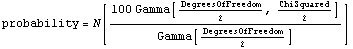
Here Gamma is a Mathematica built-in function.

As a convenience, EDA supplies a function ChiSquareProbability.
In[2]:=
In[3]:=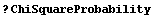
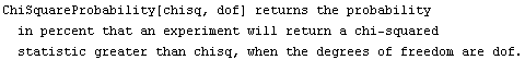
The interpretation of this statistic is a bit subtle. We assume that the experimental errors are random and statistical. Thus, if we repeated the experiment we would almost certainly get slightly different data, and we would therefore get a slightly different result if we fit the new data to the same model as the old data. As the usage message indicates, the chi-squared probability is the chance that the fit to the new data would have a larger ChiSquared than the fit we did to the old data.
If our fit returned a ChiSquared of zero, then it is almost a certainty that any repeated measurement would yield a larger ChiSquared.
In[4]:=
Out[4]=
If the ChiSquared is equal to the number of degrees of freedom, then the probability depends on the ChiSquared.
In[5]:=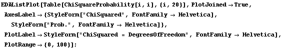
The probabilities range from 32% to 48%. These are the kinds of probabilities we would expect if our estimates of experimental uncertainties are reasonable and the data is fitting the model reasonably well.
If we have a ChiSquared of 100 for 10 DegreesOfFreedom, the probability is very small.
In[6]:=
Out[6]=
This number indicates that no repeated experiment is likely to fit so poorly to the model. The conclusion may be that the data in fact is not related to the model being used in the fit.
If the ChiSquared is much less than the DegreesOfFreedom, the fit is almost too good to be true.
In[7]:=
Out[7]=
One possibility is that the experimenter has overestimated the experimental errors in the data.
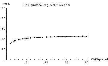
If the ChiSquared is, say, twice the number of degrees of freedom, the probability depends on the number of degrees of freedom.
In[8]:=
For two degrees of freedom the probability is 14%, which is not too unreasonable and indicates a fairly reasonable fit. For 20 degrees of freedom the probability falls to 0.5%, which indicates a very poor fit.
We summarize the use of the ChiSquared in evaluating the result of a fit.
A good fit should have a ChiSquared close to the number of degrees of freedom of the fit. The larger the number of degrees of freedom, the closer the ChiSquared should be to it.
That said, say we have good data including good estimates of its errors, and we are fitting to a model which does match the data. If we repeat the experiment and the fit many times and form a histogram of the ChiSquareProbability for all the trials, it should be flat; we expect some trials to have very small or large probabilities even though nothing is wrong with the data or the model. Thus, if a single fit has a very large or very small chi-squared probability, perhaps it is coincidental and there is nothing wrong with the data or the model. In this case, however, repeating the measurement is probably a good idea.
Despite its limitations, statistical analysis is very useful. However, one of the best ways of evaluating a fit is graphically. Supplied with EDA is a famous quartet of made up data by Anscombe that illustrates this.
In[9]:=

All data sets supplied with EDA have a usage message.
In[10]:=
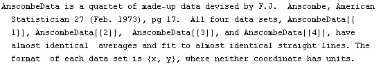
Each data set consists of 11 {x, y} pairs.
In[11]:=
Out[11]=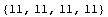
The averages of both x and y for all four are almost the same.
In[12]:=
Out[12]=
We can use the EDA function LinearFit to fit each data set to a straight line. LinearFit is introduced in the next section, and the details of options used below are not important here; for now, we simply note that the function returns the intercept and the estimated error in the intercept as a[0], and the slope and its error as a[1].
In[13]:=


The command also stored the intercept and slope of each fit in fittable.
Note that the results of these fits, including the SumOfSquares, are almost identical. So by just looking at the numbers we might conclude that all four fits are similarly reasonable.
Now we make a 2  2 matrix of graphs; each graph contains both the result of the fit to the data and the data itself. 2 matrix of graphs; each graph contains both the result of the fit to the data and the data itself.
In[14]:=
Finally, we display the graphs.
In[16]:=

Graph 1 shows that modeling AnscombeData[[1]] to a straight line is reasonable, while graph 2 shows the danger of using an incorrect model. Graphs 3 and especially 4 illustrate the fact, discussed above, that least-squares fits are not resistant to the influence of a "wild" data point.
4.1.5 References
Philip R. Bevington, Data Reduction and Error Analysis (McGraw-Hill, 1969), pp. 134 ff and 204 ff. A classic introduction to least-squares fitting.
Gene H. Golub and James M. Ortega, Scientific Computing and Differential Equations (Academic Press, 1992), pp. 89 ff and 139 ff. Another good introduction that also discusses using QR factorization.
Matthew Lybanon, American Journal Physics 51, (1984), p. 22. Discusses a modified and improved effective variance technique.
Jay Orear, American Journal Physics 50, (1982) p 912. Introduces the effective variance technique.
William H. Press, Brian P. Flannery, Saul A. Teukolsky, and William T. Vetterling, Numerical Recipes in C (Cambridge Univ., 1988), Chapter 14. The code of the LinearFit package largely uses the notation of this book, which also discusses singular value decomposition.
William H. Press and Saul A. Teukolsky, Computers in Physics 6, (1992) p. 274. A discussion of fitting when the data has errors in both coordinates, with an example of the Brent method.
J. R. Taylor, An Introduction to Error Analysis (University Science Books, 1982), p. 158 ff. A good discussion of least-squares techniques, this also discusses the "statistical assumption" used by LinearFit when the data has no errors and the Reweight option is set to True.
4.2 Curve Fitting When the Data Have No Explicit Errors
In this section we discuss the Mathematica Fit function and then introduce the EDA function LinearFit.
We will use GanglionData, which is supplied with EDA.
In[1]:=
In[2]:=

Like all data supplied with EDA, information about the data is included.
In[3]:=
We examine the data.
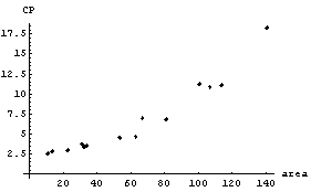
In[4]:=

In this graph, CP denotes central to peripheral cell density ratio and area denotes retinal area.
We can also use the EDA function EDAListPlot.
In[5]:=
Lia, et al., who took the data, also fit it to a straight line and from that fit deduced information about the growth of the retina.
We fit the data to a straight line using the built-in Mathematica Fit function.
In[6]:=
Out[6]=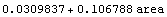
Next, we plot the result of the fit.
In[7]:=
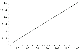
We display both the data and fit together.
In[8]:=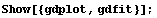
We calculate a list of the residuals.
In[9]:=
Out[9]=
For less experienced Mathematica users, this calculation is "unwound" in Section 4.2.1. We examine the residuals.
In[10]:=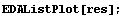
For a good fit (i.e., good data fit to a correct model) we expect the residuals to be randomly distributed about zero. This does not appear to be the case for the residuals of our straight-line fit to GanglionData.
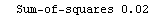
The sum of the squares of the residuals can be calculated.
In[11]:=
Out[11]=
The smaller this number, the "better" the fit.
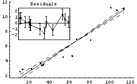
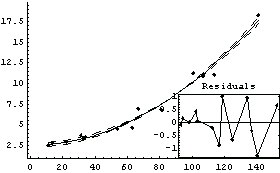
By default LinearFit, which is supplied by EDA, fits to polynomials. Using it, we can similarly fit GanglionData to a straight line.
In[12]:=
Out[12]=
The {0, 1} in the call to LinearFit tells the program that we are fitting to two parameters. The basis function of the first parameter is  , and the basis function of the second parameter is , and the basis function of the second parameter is  . The a in the call to LinearFit is an arbitrary symbol that is used the present the result of the fit. . The a in the call to LinearFit is an arbitrary symbol that is used the present the result of the fit.
By default LinearFit returns a set of rules. The first rule states that the value of the parameter for a[0], the intercept, is 0.03; LinearFit has also estimated the error in that parameter to be ± 0.72. The second rule states that the value of the parameter for a[1], the slope, is 0.107 ± 0.01. The function also returns the SumOfSquares and the DegreesOfFreedom.
LinearFit has used a "statistical assumption" about the errors in the independent variable of the dataset and returns the value of that error as PseudoErrorY. The behavior can be controlled with the Reweight option discussed in Section 4.4.1.13.
Note that by default LinearFit displays some graphical information about the fit. The large graph displays the data and the results of the fit; since the parameters of the fit have errors, these maximum and minimum values of the fit are also displayed. The small insert also displays the residuals; this plot seems to confirm the indication of the previous residual plot for this data that the data point for the largest area is pulling the value of the slope up from the value consistent with the other data.
This graphic object is not returned by LinearFit; the function returns the numerical rules only.
In[13]:=
Out[13]=
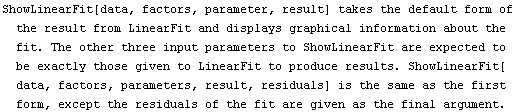
The ShowLinearFit function, which is used internally by LinearFit, can be accessed directly and does return the graphic object. Section 4.4.2.1 provides further details.
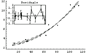
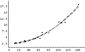
Perhaps the suspicious appearance of the residual plot is not due to a slightly wild data point; maybe the model that CP versus area is linear in area is incorrect. Let's look at a fit to a second-order polynomial.

In[14]:=

Out[14]=
The graph indicates no systematic problems with the residuals. However, note that the error in the slope a[1] is larger than the value of the slope itself.
The fact that the errors in the a[1] term are larger than the value of the a[1] term suggests that perhaps we should be fitting to a parabola.
Doing the fit seems to affirm that suggestion.
In[15]:=
Out[15]=
It is tempting to accept this as the "best" fit to the data. We will find yet another good fit to the data in Section 8.2.1.
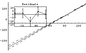
It is important to emphasize that the above analysis, although suggestive, certainly does not prove that this data should not be modeled by a straight line. Many of the problems with the straight-line fit were due to the last data point. We repeat some of the fits we have just done, but this time dropping that data point.
In[16]:=
Out[16]=
In[17]:=
Out[17]=
Now it is much more difficult to choose between the two models, although the only difference is one data point. The residuals for the straight-line fit still look slightly suspicious, and the SumOfSquares for the second fit is about half the values for the straight-line fit. As we have already stated, analyzing the fit of data to a model is sometimes very subtle.
As mentioned, Lia et al. used their straight-line fit to deduce information about the growth of the retina. Cleveland is certainly harsh when he states, "Astonishingly, the three experimenters who gathered and analyzed the data, fitted a line." (Reference: William S. Cleveland, Visualizing Data (AT&T Bell Laboratories, 1993), p. 91). You may, of course, explore this data further and draw your own conclusions.
We will explore the ganglion data further in Sections 6.1.3, 6.2.3, 7.1.1, and especially in 8.2.1.
4.2.1 Unwinding the Residual Calculation
The residual was calculated in the previous section.
 Here the command is "unwound" for less experienced Mathematica users. First, look at the data itself.
In[18]:=
Out[18]=
Then we extract the independent variable, area.
In[19]:=
Out[19]=
Similarly, we extract the dependent variable, CP.
In[20]:=
Out[20]=
The variable result is the result of using Fit.
In[21]:=
Out[21]=
We can evaluate the value of CP predicted by this fit for each value of area.
In[22]:=
Out[22]=
We subtract these values from the experimental values of CP.
In[23]:=
Out[23]=
These are the residuals for each data point. Finally, we form a list where each element is {area, residual}.
In[24]:=
Out[24]=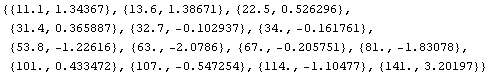
This is the command we have been unwinding.
Often a command such as this is written by building up to it in stages often identical to the way we have unwound it.
4.3 Curve Fitting When the Data Have Explicit Errors
In this section we discuss fitting to data where the experimenter has provided errors in one or both of the coordinates.
We begin by looking at calibration data for a thermocouple, a temperature measuring device.
In[1]:=
In[2]:=

In[3]:=
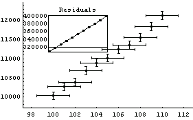
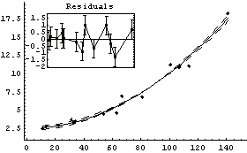
We begin by fitting the data to a straight line.
In[4]:=
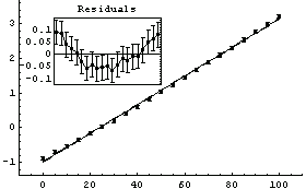
Out[4]=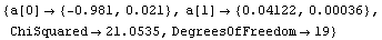
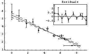
Although the errors in the fitted parameters, the ChiSquared per DegreesOfFreedom, the plot of the data, and the results of the fit all look fairly reasonable, the plot of the residuals shows clearly that something is wrong with this fit.
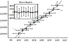
We fit to the data again, this time adding a quadratic term.
In[5]:=

Out[5]=
Now the residuals appear to have zero slope, and the errors in the fitted parameters are all smaller than the values of those parameters. However, the ChiSquared is much smaller than the DegreesOfFreedom. This appears too small and, in fact, the probability is essentially 100%.
In[6]:=
Out[6]=
The data was taken by Bevington and when we examine the details of how he collected the data, we discover that his claimed errors are not an estimate of his reading error or the amount of fluctuation of the needle of the voltmeter. Rather they are just a guess made by the experimenter. The ChiSquareProbability indicates that the guess was fairly pessimistic.
Not only was Bevington careful enough to supply the above information, he also tells us that the measurements were made on two scales of the voltmeter, the 1 mV and the 3 mV scales. Let us assume that the error of precision, either due to reading error or fluctuations in the needle, is 1% of the value of the scale being used. We can form a new data set using these errors.
In[7]:=
A fit to a second-order polynomial looks more reasonable.
In[8]:=
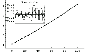
Out[8]=
In[9]:=
Out[9]=
Comparing the values of the parameters of the fit to the ones we obtained using Bevington's original errors in the voltage, we see that the values have changed somewhat but the two fits are the same within estimated errors in those parameters. Further, the errors in the parameters for this second fit are, perhaps expectedly, much smaller than for the first. It may be reasonable to use this fit as our "final" calibration result.
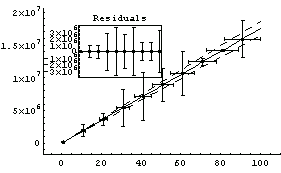
LinearFit can also handle data in which there are errors in both coordinates. Pearson's data from 1901 with York's weights, although made up and not from a real experiment, are often used to test fitters.
In[10]:=

In[11]:=

We fit PearsonYorkData to a straight line.
In[12]:=
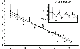
Out[12]=
In this fit an "effective variance technique" discussed in Section 4.1.3 has been used.
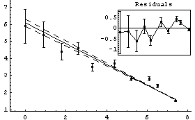
One of the features of the errors in the coordinates that makes these fits interesting to statisticians is that for small values of x the error in y dominates, while for large x it is the error in x that dominates. An option to LinearFit allows us to examine the values of the effective variance; we also use the ShowFit option to suppress the graphs of the fit.
In[13]:=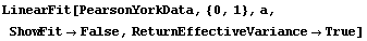
Out[13]=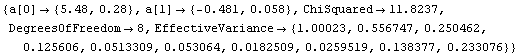
Note that the square root of the effective variances are the errors in the dependent variable used by LinearFit.
We can also examine the effect of these errors in the independent variable on the fit by forming a data set containing only the error in the dependent variable and fitting to a straight line.
In[14]:=
In[15]:=
Out[15]=
The ChiSquared is large compared to the DegreesOfFreedom. In fact, it is difficult to find a fit to newData with a reasonable ChiSquareProbability. The following tries a number of powers and prints the probability.
In[16]:=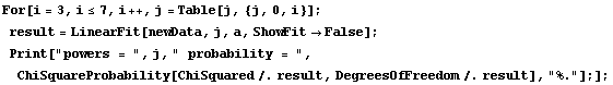


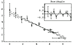
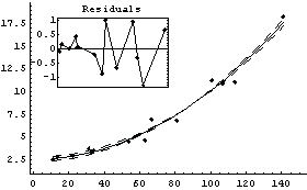
We end this section by looking at some real data for a plastic ball in free fall.
In[17]:=

In[18]:=
Without air resistance we expect the distance s to be related to the time t according to a second-order polynomial.
Therefore, we try a second-order polynomial first.
In[19]:=
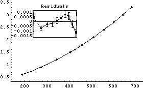
Out[19]=
The ChiSquared per DegreesOfFreedom is large. In addition, there is a clear sign of a systematic problem in the residuals.
One simple, but approximate, way to incorporate the effects of air resistance on this data is to add a cubic term to the polynomial.
In[20]:=
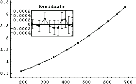
Out[20]=
The a[2] term should be nearly equal to 1/2 g, where g is the acceleration due to gravity. From this experiment, then, g can be calculated.
In[21]:=
Out[21]=
This is in m per  . We re-cast as m per . We re-cast as m per  . .
In[22]:=
Out[22]=
Thus, Professor Key has performed a better than 1% determination of g. In the location in Toronto where this data was collected, the accepted local value of g is 9.8012 ± 0.0010 m/ , which is consistent with this result. , which is consistent with this result.
4.4 Options, Utilities, and Details
This section discusses the LinearFit package in more detail.
There are many options to LinearFit that control both how it performs the fit, and what values and formats it returns; these are discussed in Section 4.4.1.
The LinearFit package also includes functions that are used by LinearFit but may also be used directly; these are the topic of Section 4.4.2.
First we load EDA.
In[1]:=
4.4.1 Options to LinearFit
These are the options to LinearFit and their default values.
In[2]:=
Out[2]//TableForm=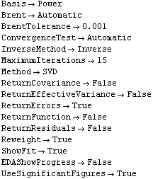
Below we discuss these in order.
The default values of these options have been set so that LinearFit will do the "right thing" for most simple analysis problems, while providing sufficient flexibility for more sophisticated problems.
In addition, if ShowFit is set to True (the default) LinearFit uses the function ShowLinearFit. This function is discussed in Section 4.4.2. Options to ShowLinearFit given to LinearFit are passed to that function.
If LinearFit is called with ReturnFunction set to True, or the ShowFit option is set to True (the default) then the function ToLinearFunction is called; this function is also discussed in Section 4.4.2. Options to ToLinearFunction given to LinearFit are passed to that function.
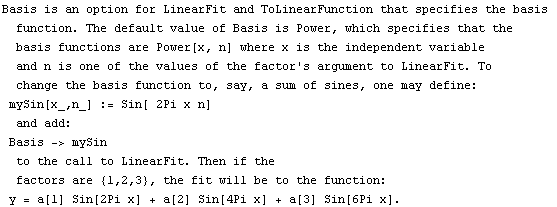
4.4.1.1 The Basis Option
The default basis function for LinearFit is the Mathematica function Power, which causes LinearFit to fit to polynomials. It may be changed to a user-supplied function using the Basis option.
In[3]:=

Our first illustration will use some made-up data that is a linear combination of three Bessel functions with a small noise.
In[4]:=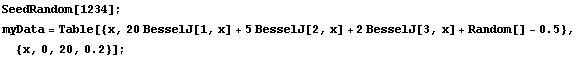
The order of the input arguments to BesselJ is the reverse of what we require for LinearFit, so we define a convenience function myBesselJ.
In[6]:=
Now we can fit to the data.
In[7]:=
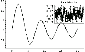
Out[7]=
Finally, we illustrate the Basis option with some real mass spectrometer data.
In[8]:=

In[9]:=
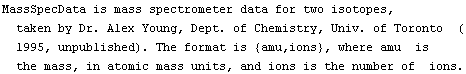
In[10]:=
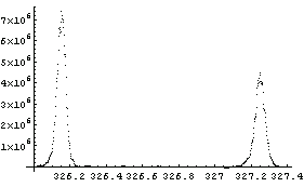
After folding in calibration and resolution numbers from the mass spectrometer, the two peaks can be approximated as Gaussians. The center of the first peak is 326.155 amu with standard deviation 0.0240 amu; the center of the second peak is 327.255 amu with a standard deviation of 0.0276 amu. These values are included in the following definition of the basis function.
In[11]:=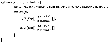
Note that the input arguments are the same as for Power: the first is the value of the independent variable and the second is the factor.
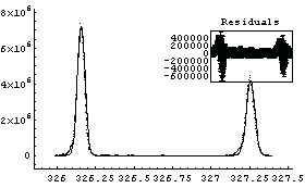
We fit the MassSpecData.
In[12]:=
Out[12]=
The residuals show that modeling this spectra as Gaussians is not perfect.
Note also that this is a linear fit, since we are only fitting to the amplitudes of the two peaks: to fit to the center values and/or widths of the peaks would require using FindFit, which is discussed in Chapter 5.
4.4.1.2 The Brent Option
For fitting to a straight line with powers {0, 1}, if there are errors in both coordinates and the ReturnCovariance option discussed below is set to False (the default) then, by default, LinearFit uses a Brent minimization algorithm.
We begin by repeating a fit we have done before.
In[13]:=
Out[13]=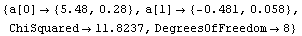
The algorithm used here differs from the "standard" one that we see in many references, in which one simply iterates the solution recalculating the effective variance at each iteration. This "standard" technique may be used by setting Brent to False.
In[14]:=
Out[14]=
For this data the exact solutions are known. The intercept is 5.47991025 and the slope is -.480533415.
Notice that both methods return the same values within their claimed errors, and they are both within errors of the exact values, although the Brent algorithm gives results that are closer.
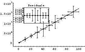
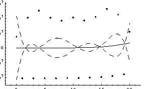
For lines with very large slopes, Brent tends to do a more realistic job of estimating the errors in the fitted parameters. We illustrate with some made-up data, mydata.
In[15]:=
Compared to Brent's calculation, the non-Brent method seems to have errors that are too small.
In[17]:=
Out[17]=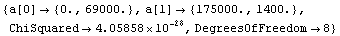
In[18]:=
Out[18]=
The disadvantages of the Brent method are: (1) it is only available for straight-line fits, (2) it is about an order of magnitude slower than the standard method, and (3) it cannot return the full covariance matrix. We illustrate the last point using the ReturnCovariance option discussed below.
In[19]:=
Out[19]=
The central idea of the Brent algorithm is that we weight the sum of the squares of the residuals with the effective variance errors.
Here the Xs are the basis functions and the effvar is the effective variance error. In general, this is not linear in the parameters to which we are fitting. But in the case of a straight line, the derivative of the sum of the squares with respect to the intercept is linear, and we can set the derivative to zero.
For further information on this algorithm, see Press and Teukolsky, Computers in Physics 6, (1992), p. 274.
4.4.1.3 The BrentTolerance Option
The tolerance used by Brent minimization is controlled by the BrentTolerance option. We examine once again the fit to PearsonYorkData, this time turning off significant figure adjustment in the result using the UseSignificantFigures option discussed below.
In[20]:=
Out[20]=
The values compare well with the known exact solution, which is an intercept of 5.47991025 and slope of -.480533415.
We can decrease the tolerance used by the Brent minimization from its default value of 0.001.
In[21]:=
Out[21]=
This yields an answer a bit closer to the exact values. Considering the size of the calculated errors in the fit parameters, these two results are essentially the same.
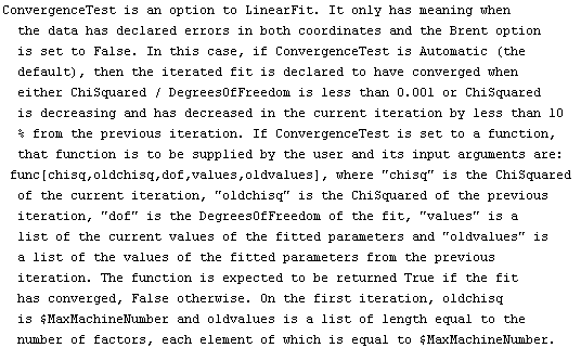
4.4.1.4 The ConvergenceTest Option
The ConvergenceTest option allows the user to control when the fit is considered to have converged.
In[22]:=

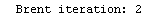
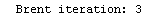
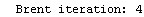
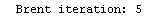
For example, here is a fit we have performed before, but this time we use the EDAShowProgress option discussed below to follow its progress.
In[23]:=


Out[23]=
Say we decide that the convergence test will be when the maximum change in the values of the fitted parameters is less than 10% of those of the previous iteration. Then we can define a routine for that test.
In[24]:=
In[25]:=


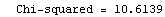


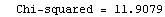


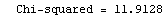
Out[25]=
This time LinearFit has decided that the fit converged after three iterations, instead of the five iterations before.
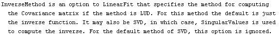
4.4.1.5 The InverseMethod Option
When the method of doing the fit is LUD (cf. the b option below), then the calculation of the covariance matrix by default uses Mathematica's Inverse function.
Sometimes, this calculation is not stable. If InverseMethod is set to SVD, then singular value decomposition is used instead of Inverse; this will often be more stable.
Reference: J. Stoer and R. Burlisch, Introduction to Numerical Analysis (Springer, 1980).
For example, we will fit to the thermocouple data we examined in Section 4.3.
We will fit it to a cubic polynomial, using the LUD method discussed in Section 4.4.1.7.
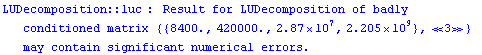
In[26]:=

Out[26]=
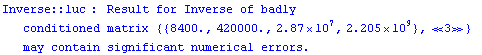
The warning message from LUDecomposition and its significance are discussed in Section 4.4.1.7. We can use a singular value decomposition (SVD) to calculate the inverse.
In[27]:=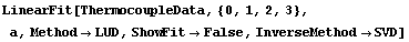
Out[27]=
This hasn't affected the complaint from LUDecomposition, but it has removed the one from Inverse.
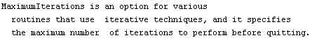
4.4.1.6 The MaximumIterations Option
The only time LinearFit iterates in performing a fit is when the data has errors in both coordinates. In this case, if the fit has not converged in MaximumIterations, the fit stops and a warning message is generated. Experience has shown that very rarely will a fit require a default value of MaximumIterations equal to 15. Nonetheless, the limit may be increased if required.
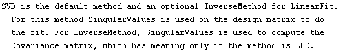
4.4.1.7 The Method Option
By default, LinearFit uses SingularValues on the "design matrix". This is not the way least-squares fits are commonly performed. Typically, they involve solving the "normal equations" of the system.
The problem with the common technique is that sometimes the data does not allow one to distinguish between two or more of the basis functions. When this occurs, the normal equations become nearly singular and the solutions are unstable.
When the Method option is set to LUD, the common algorithm is used, involving LU decomposition of the normal equations.
For example, we can fit the ThermocoupleData that we used in Section 4.3 to a cubic polynomial.
In[28]:=
Out[28]=
Note that a[3] is not only very small but is zero within errors. We can use the common least-squares method.
In[29]:=


Out[29]=
In this case, despite the warnings from LUDecomposition, the result of the fit came out the same. This will not necessarily always occur.
Regarding the complaint from Inverse in this fit, see the discussion of the InverseMethod option in Section 4.4.1.5.
Often, as in the example shown, the reason for the complaint from LUDecomposition is that inherent in the least-squares algorithm is an assumption that the basis functions are orthogonal. If this is not true, then one or more of the pivot elements of the "normal equations" of the problem will be very small. More often than many experimenters would like to admit, the data does not allow one to justify the assumption that the basis functions are orthogonal.
Finally, if we are fitting data to a line with the slope forced to zero, the default SVD method does not work. In this case LinearFit automatically changes to LUD; this change is done silently unless the EDAShowProgress option is set to True.
In[30]:=


Out[30]=
4.4.1.8 The ReturnCovariance Option
The square root of the diagonal terms of the covariance matrix are the errors in the fitted parameters. LinearFit assumes that the off-diagonal terms of the covariance matrix are small, which means that the correlation between fitted parameters are similarly small.
By setting ReturnCovariance to True, the full covariance matrix is returned so that this assumption can be checked. For example, we use ThermocoupleData, which was discussed in Section 4.3, and have LinearFit return the covariance matrix.
In[31]:=
Out[31]=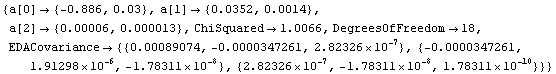
We can see the matrix more clearly using MatrixForm.
In[32]:=
Out[32]//MatrixForm=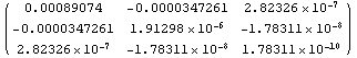
The (1, 1) term, representing the error in a[0], is the largest in the first row. Similarly, the (2, 2) term, representing the error in a[1], is larger than the (2, 3) term. So in this case the assumption of LinearFit appears to be reasonable; this will not always be true.
Also, there are occasions where the result we are trying to get from a fit involves combinations of the fitted parameters, in which case the full covariance matrix is required to calculate errors in that result. ReactanceData provides an example.
In[33]:=

In[34]:=
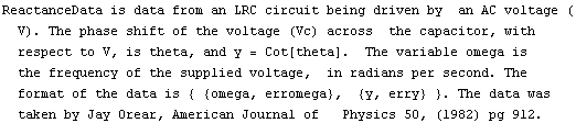
The theoretical model for this data involves two terms.
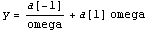
We will fit to this, setting ReturnCovariance to True and also setting the UseSignificantFigures option that is discussed in Section 4.4.1.16 to False.
In[35]:=
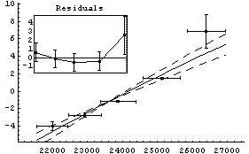
Out[35]=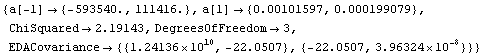
Here the off-diagonal terms of the covariance matrix are large. We will store this matrix in the variable cov for future use.
In[36]:=
Out[36]=
The two numbers desired from this experiment are the resistance r and inductance ind of the circuit. The resistance is given symbolically.
In[37]:=
Out[37]=
Here c = 0.02  F. Note that we have evaluated this definition with the Mathematica kernel because we will be using it later. F. Note that we have evaluated this definition with the Mathematica kernel because we will be using it later.
We can evaluate the resistance and its error using the Datum construct introduced in Chapter 3.
In[38]:=
Out[38]=
The units of rValue are ohms.
The inductance is given next.
In[39]:=
Out[39]=
Note that the value of ind depends on both a[1] and through r on a[-1].
If the off-diagonal terms of the covariance matrix were negligible, we could evaluate the value of the inductance and its error using simple propagation of errors.
In[40]:=

The value of the inductance above is correct, but its error is wrong because the off-diagonal term of the covariance is not negligible. We will store the value of the inductance for future use.
In[41]:=
Out[41]=
Let us rewrite the error in the resistance in terms of the covariance matrix. First, recall the definition of r.
In[42]:=
Out[42]=
Here is its derivative with respect to a[-1].
In[43]:=
Out[43]=
The value of the derivative can be calculated.
In[44]:=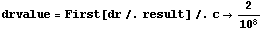
Out[44]=
The error in the value of r can be calculated.
In[45]:=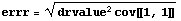
Out[45]=
Note that this is the value we got before, except the significant figures here have not been adjusted.
We can similarly duplicate the wrong value for the error in the inductance by taking the derivatives of ind with respect to both a[-1] and a[1], squaring each and multiplying by the corresponding diagonal term from the covariance matrix, adding, and taking the square root.
In[46]:=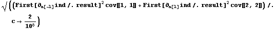
Out[46]=
However, when the "cross" term involving the off-diagonal term is added, we get an added term.

We now evaluate this expression.
In[47]:=
Out[47]=
So we achieve our final result, using an EDA function to adjust the significant figures. We first calculate the value and error in the inductance, indValue, and then list the value and error in the resistance, rValue.
In[48]:=
Out[48]=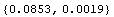
In[49]:=
Out[49]=
The units of these are henrys and ohms, respectively.
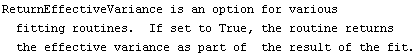
4.4.1.9 The ReturnEffectiveVariance Option
When both coordinates of the data have errors, LinearFit by default uses an "effective variance" technique. When ReturnEffectiveVariance is set to True, the final values of the effective variances are returned by LinearFit. An example of using this option appears in Section 4.3.
4.4.1.10 The ReturnErrors Option
In all the examples in sections 4.2 and 4.3, LinearFit returns not only the values for the parameters of the fit but also the estimated errors in those parameters.
When ReturnErrors is set to False, the errors are not returned. First, we repeat a fit from Section 4.3.
In[50]:=

Out[51]=
In[52]:=
Out[52]=
In the second fit, no errors in the fit parameters have been calculated. As discussed further in Section 4.4.1.16, LinearFit has also returned more significant figures in the fit parameters.
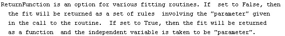
4.4.1.11 The ReturnFunction Option
The ReturnFunction option, if set to True, causes LinearFit to return a function with the parameter set to the independent variable instead of a set of rules for the fitted parameters. First, we repeat a fit from Section 4.2.
In[53]:=
Out[53]=
We repeat the fit using the ReturnFunction option.
In[54]:=
Out[54]=
The first function returned is the one that best fits the data. The second function is the estimated error in the function.
We can set ReturnFunction to True and ReturnErrors, discussed in the previous section, to False.
In[55]:=
Out[55]=
This duplicates the behavior of the built-in Fit function.
In[56]:=
Out[56]=
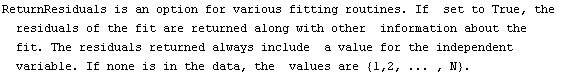
4.4.1.12 The ReturnResiduals Option
The ReturnResiduals option, if set to True, causes LinearFit to explicitly return the residuals of the fit. First, we repeat a fit from Section 4.3, using the ShowFit option discussed in Section 4.4.1.14 to suppress the graphics for the fit.
In[57]:=

Out[58]=
We once again set ReturnResiduals to True.
In[59]:=
Out[59]=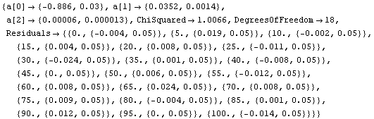
We plot the residuals.
In[60]:=
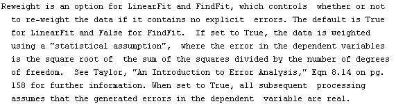
4.4.1.13 The Reweight Option
When the data has no explicit errors, LinearFit by default performs a standard minimization of the sum of the squares of the residuals. However, if the scatter in the data points can be considered to be random and statistical, then it is often reasonable to assume that the effective error in the dependent variable is the following.
By default LinearFit uses this assumption. In this case LinearFit will return, as part of the fit, the PseudoErrorY value used.
An example using this option appears in Section 4.2.
Although linear fits do not need to iterate a solution unless both coordinates have errors, LinearFit actually uses two iterations when Reweight is set to True. The first is required to calculate the PseudoErrorY, which is then used for the second and final iteration.
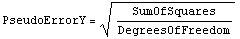
Note that internally LinearFit treats PseudoErrorY as a "real" experimental error. However, it does not return the ChiSquared, since it is always exactly equal to the DegreesOfFreedom. Instead, it returns the SumOfSquares.
Experience has shown that for most experimental data in the sciences and engineering, this default behavior is reasonable.
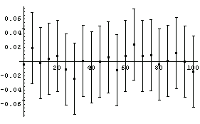
We will illustrate with some data from an experimental determination of the temperature of absolute zero.
In[61]:=

In[62]:=
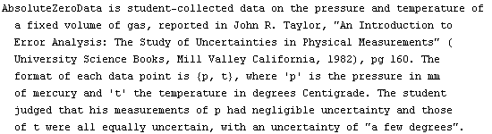
In[63]:=
Out[63]=
The fit gives a value for absolute zero of -263 ± 18 degrees centigrade; the accepted value of -273 degrees centigrade is well within this range. Also, the value of the PseudoErrorY is consistent with the student's estimate of an error of "a few degrees" in the temperature.
We repeat the fit without reweighting.
In[64]:=
Out[64]=
The only effect of setting Reweight to False is in the errors in the fitted parameters; the significant figure adjustment discussed in Section 4.4.1.16 makes that somewhat less than obvious in the above result, but it is in fact true. For this fit, the effect is to reduce the errors in the parameters, making the experimental result for absolute zero equal to -263.3 ± 2.7 degrees centigrade, which is significantly different than the accepted value of -273 degrees.
In general, experience with a wide range of experimental data from a variety of fields of science and engineering has shown that the default setting of Reweight to True is almost always the most reasonable one for linear fits.
4.4.1.14 The ShowFit Option
As discussed in some of the sections above, if the ShowFit option is set to False, the graphical display of information about the fit is not shown. In this case, the information returned by LinearFit can be used later to create the graphical display by using the ShowLinearFit function discussed in Section 4.4.2.
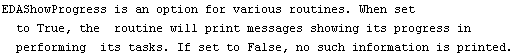
4.4.1.15 The EDAShowProgress Option
When the EDAShowProgress option is set to True, LinearFit prints some information about its progress as it does its work. For example, we repeat a fit that was done in Section 4.3 but will turn on the EDAShowProgress option.
In[65]:=


Out[65]=
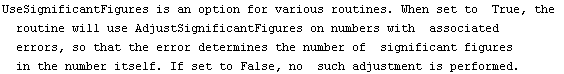
4.4.1.16 The UseSignificantFigures Option
As discussed in Chapter 3, in the physical sciences a specification of an error associated with a quantity essentially defines what the significant figures of that quantity are. By default, LinearFit uses this definition of significant figures in returning the values of the fit parameters. For example, here we repeat a fit we have already done a few times in this subsection.
In[66]:=
Out[66]=
Setting UseSignificantFigures to False yields more digits in the fit parameters.
In[67]:=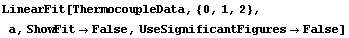
Out[67]=
Now the estimated errors in the fitted parameters have not been used to adjust the number of significant figures displayed for either the values or the errors in those parameters.
Sometimes, when the model being used is extremely poor for the data, a very high error is returned for one or more of the fit parameters. In this case, adjustment for significant figures can turn the value to zero. For example, here is some made-up data for a parabolic relation.
In[68]:=
Out[69]=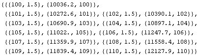
We attempt to fit this to a model.
In[70]:=
Out[70]=
Here the wild value for the intercept means that the curve representing the fit doesn't even appear on the graph! Turning off significant figure adjustment makes things more reasonable for this unreasonable fit.
In[71]:=
Out[71]=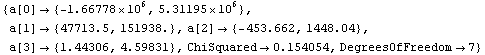
Turning off significant figure adjustment can be required in other contexts. For example, WamplerData is synthetic data used to test least squares fitters.
In[72]:=
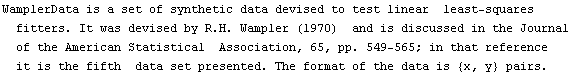
The certified regression statistics for this data, when it is fit to a fifth order, polynomial are as follows.
a[0]  {1.00000000000000 ,21523262.4678170} {1.00000000000000 ,21523262.4678170}
a[1] {1.00000000000000 , 23635517.3469681
a[2] {1.00000000000000 , 7793435.24331583}
a[3] {1.00000000000000 , 1014755.07550350}
a[4] {1.00000000000000 , 56456.6512170752}
a[5] {1.00000000000000 ,1123.24854679312}
Notice that the errors in all six parameters are much larger than the value of the corresponding parameter; if this was a fit to real experimental data we would almost certainly interpret this to mean that all six parameters are zero within errors. LinearFit will, reasonably, return values consistent with this interpretation.
In[73]:=
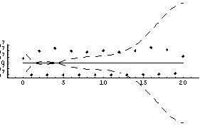
Out[73]=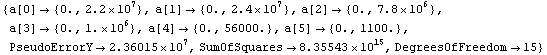
In order to compare LinearFit to the certified results of the regression for this data, we turn off significant figure adjustment.
In[74]:=
Out[74]=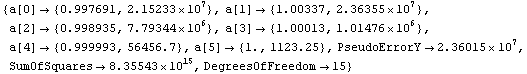
This result shows good agreement with the certified results.
The National Institutes of Standards and Technology (NIST) has a large collection of data, including WamplerData, for testing fitters at their web site http://www.itl.nist.gov/div898/strd/.
4.4.2 Other Routines in the LinearFit Package
4.4.2.1 The ShowLinearFit Routine
LinearFit uses ShowLinearFit to display the results of a fit. If we have the results of LinearFit, we can use ShowLinearFit to display it. We will demonstrate with the GanglionData used in Section 4.2.
In[75]:=
Out[75]=
Now we display the results of the fit.
In[76]:=
Out[76]=
Note that ShowLinearFit returns a Graphics object. This can be convenient if you wish to print the graphic, since the Graphics object is not returned by LinearFit itself.
If LinearFit has used a Basis other than the default, this option should be included in the call to ShowLinearFit also.
Although the symbol a is arbitrary in the call to LinearFit, the symbol in the call to ShowLinearFit must be the same as that used in the call to LinearFit; this is because that symbol is used in result.
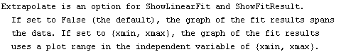
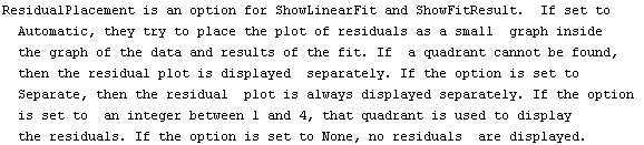
ShowLinearFit by default tries to find a quadrant in the data-fit graph in which to place the residual plot; if no such quadrant can be found, the residual plot is displayed separately. Setting ResidualPlacement to Separate causes the residual plot to always be displayed separately. ResidualPlacement can also be set to an integer between 1 and 4, which causes the residual plot to be placed in that quadrant of the data-fit plot.
In[77]:=
Out[77]=
If ResidualPlacement is set to None, no residual plot is displayed.
In[78]:=
Out[78]=
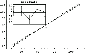
By default, the plot of the fit results spans the experimental data. An Extrapolate option causes the values of the independent variable to be the range specified by the option. For example, here is a fit to data from a constant-volume gas thermometer.
In[79]:=

Out[79]=
The value of the intercept is absolute zero in Celsius. The numerical fit results indicate a value for this of -263 ± 18 C, but the graph does not show the intercept. We now extrapolate the fit results.
In[80]:=
Out[80]=
Internally, ShowLinearFit uses EDAListPlot, Plot, and ToLinearFunction. Options given to ShowLinearFit for these are passed to the appropriate function. The only option used directly by ShowLinearFit is ResidualPlacement.
There can be some minor differences between the graphs displayed by LinearFit and those displayed by ShowLinearFit. For example, if the data set has no explicit errors and the Reweight option is set to True (the default), then the PseudoErrorY is used in the calculation of the errors in the residuals by LinearFit. ShowLinearFit is unaware of this and will then show no errors in the residual graph. By specifying ReturnResiduals to be True in the call to LinearFit, the "better" numbers will be used by ShowLinearFit.
For example, here is the fit to GanglionData once again.
In[81]:=

Out[81]=
We use ShowLinearFit on result.
In[82]:=

ShowLinearFit does not show the errors in the residuals due to the PseudoErrorY term.
Now we have LinearFit explicitly return the residuals.
In[83]:=
Out[83]=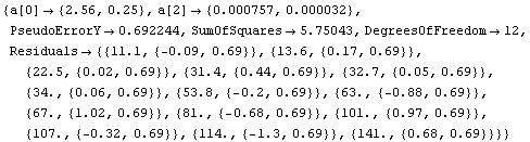
We can see that the PseudoErrorY has led to an error in each of the residuals. ShowLinearFit will display these in this case.
In[84]:=
Similarly, if the data set has errors in both coordinates, LinearFit uses the effective variance in calculating the errors in the residuals. In this case also, specifying ReturnResiduals to be True in the call to LinearFit will cause ShowLinearFit to be slightly more correct.
Finally, when LinearFit itself calls ShowLinearFit, with errors in the fit parameters that are to be displayed in the plot, the calculation of those errors involves using the covariance matrix which is automatically passed to ShowLinearFit. If the covariance matrix is not explicitly returned in the result of the fit, a heuristic technique is used to calculate the errors, which may give a different result. The actual calculation of those errors is done by the ToLinearFunction function discussed in the following subsubsection.
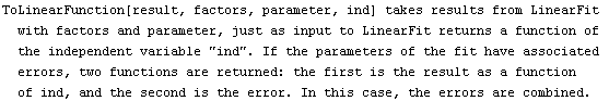
4.4.2.2 The ToLinearFunction Routine
ShowLinearFit, discussed in the previous subsection, uses the function ToLinearFunction to graph the results of the fit. LinearFit also directly calls ToLinearFunction if the option ReturnFunction is set to True.
The function may also be called directly. We repeat a fit we have done before.
In[85]:=
Out[85]=
We give result to ToLinearFunction.
In[86]:=
Out[86]=
The first function is the fit, using temperature as the name of the independent variable. The second is the estimated error function due to the errors in the fitted parameters.
Although the name a is arbitrary in the call to LinearFit, it must be the same name in the call to ToLinearFunction, since it is contained in result.
If the Basis is changed in the call to LinearFunction, the same Basis option should be used in the call to ToLinearFunction.
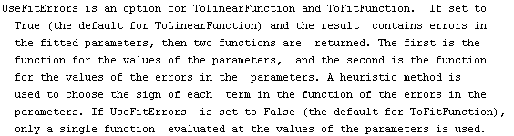
Finally, when called from LinearFit, either because ShowFit is set to True (the default) or ReturnFunction is set to True and the UseFitErrors option to ToLinearFunction is set to True (the default), the calculation of those errors involves using the covariance matrix.
When ToLinearFunction is called separately and the covariance matrix is not part of the result from LinearFit, a heuristic technique is used to calculate the error function.
We fit ThermocoupleData to a second-order polynomial and use the result to form a function with ToLinearFunction.
In[87]:=
Out[87]=
In[88]:=
Out[88]=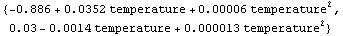
Note that the terms in the second function alternate. The heuristic that decides on the sign of each term follows.
1. Calculate the value of each of the basis functions at the somewhat arbitrary value of the independent variable of 10.
2. Sort these values.
3. Error terms that correspond to odd-numbered positions in the sorted list will have positive coefficients. Terms that correspond to even-numbered positions in the sorted list will have negative coefficients.
Experience has shown that this heuristic is often reasonable. However, returning an error function can be turned off as follows.
In[89]:=
Out[89]=
4.5 Summary of the LinearFit Package
In[1]:=
4.5.1 The LinearFit Routine
In[2]:=
In[3]:=
Out[3]//TableForm=
In[4]:=

In[5]:=

In[6]:=
In[7]:=
In[8]:=
In[9]:=
In[10]:=
In[11]:=

In[12]:=

In[13]:=

In[14]:=
In[15]:=

In[16]:=
In[17]:=
In[18]:=
In[19]:=

In[20]:=
In[21]:=
4.5.2 The ShowLinearFit Routine
In[22]:=
ShowLinearFit uses options from ListPlot, MultipleListPlot, and Plot. It also has the following specific options.
In[23]:=
In[24]:=
In[25]:=
In[26]:=

4.5.3 The ToLinearFunction Routine
In[27]:=
In[28]:=
Out[28]//TableForm=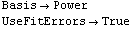
In[29]:=

In[30]:=
|