Chapter 1

Introduction to Experimental Data Analyst

Experimental Data Analyst (EDA) is a collection of tools and tutorials designed specifically for the needs of physical scientists, engineers, and students of science and engineering. Included are over 30 functions, tutorials in using the functions, tutorials in using Mathematica built-in commands and standard Mathematica packages, and discussions of the underlying theory of data analysis at a variety of levels from beginning undergraduate to practicing researcher. The tutorials make use of a variety of real experimental data drawn from many different fields, and the data is also included in the package.

The material is divided into eight chapters, beginning with this chapter, which provides an overview of the contents. The chapters can be accessed as a hard-copy version or read online as Mathematica notebooks. The notebooks can be read with the front end included with Mathematica or with the free MathReader program available from www.mathreader.com; in the former case, the notebooks can be interactive, and the reader is encouraged to experiment with the commands and supplied data sets.

The chapters do not all have to be read in order. In general, we recommend that you look over this chapter in its entirety before going on to the others. Section 1.1.1 gives further recommendations of which chapters and sections are probably prerequisites for succeeding ones.

1.1 Summary and Use of EDA

1.1.1 Summary of the Chapters of EDA

Chapter 2 deals with methods of getting data into Mathematica so that it may be analyzed. This chapter is independent of all other chapters included with EDA. It discusses techniques to read and write files containing data sets and also introduces the EDA programs ImportData and ExportData.

Chapter 3 discusses a topic which pervades data analysis in the physical sciences and engineering: error analysis. Here a tutorial is supplied. Although the level is suitable for an undergraduate student in the sciences, we are also aware of many professional researchers whose education and training have managed to miss some of the material discussed here. In addition, EDA supplies programs and constructs to simplify error analysis, and they are introduced in this chapter. The EDA functions discussed are AdjustSignificantFigures, CombineWithError, DivideWithError, PlusWithError, PowerWithError, Quadrature, SubtractWithError, and TimesWithError. Also, EDA defines Data and Datum constructs for doing propagation of errors; these constructs are introduced in this chapter. The functions and constructs discussed here are used in later chapters.

Chapters 4 through 8 are the "heart" of the analysis tools provided by EDA.

Chapter 4 introduces one of the most commonly performed tasks in data analysis: fitting data to linear models, especially straight lines and curves. Section 4.1 provides background discussions of a linear fit, least-squares techniques, evaluation of the quality of the fit, etc.; some familiarity with this material is assumed in all later sections. The remainder of Chapter 4 discusses the EDA function LinearFit, which performs linear least-squares fits to data. Included is a discussion of the related EDA functions ShowLinearFit and ToLinearFunction. The LinearFit function is used in all subsequent chapters. Also, many other EDA functions have similar syntax. Thus, some familiarity with its syntax and options is recommended.

Chapter 5 extends the materials of Chapter 4 to arbitrary models. It introduces the EDA function FindFit and the related functions ShowFitFunction and ToFitFunction. Also discussed are some convenience functions that define peak shapes; these are BreitWigner, Galatry, Gaussian, Lorentzian, PearsonVII, RelativisticBrietWigner, and Voigt. Most of the information in this chapter is not used in later discussions, although the FindPeaks function discussed in Chapter 8 is primarily intended as a companion to FindFit.

Chapter 6 discusses techniques to eliminate noise in data and to fill in missing values. It also discusses the related topic of fitting data when a model is not available or appropriate. The chapter introduces the EDA functions SmoothData, LoessFit, and FillData. There is also a tutorial on using built-in Mathematica functions to smooth data, and the algorithm used by the FindPeaks program discussed in Chapter 8 is introduced here. With the exception of the algorithm of FindPeaks, nothing in later chapters depends on anything appearing here.

Chapter 7 discusses techniques to fit data to lines and curves when one or more of the data points may be "wild", that is the data contains "outliers." Alternatives to least-squares techniques should be considered in this case since an outlier can have a significant effect on the least-squares fit. The chapter introduces the EDA functions RobustCurveFit and RobustLineFit. Nothing in the chapter is required for Chapter 8.

Chapter 8 discusses what to do when the relations in a data set are not known. Graphical techniques are explored in Section 8.1. The discussion includes the EDA function EDAListPlot, which is briefly introduced in Section 1.3 and the EDA functions EDAHistogram and BoxPlot are also discussed. Section 8.2 is a tutorial on using Mathematica built-in functions to transform the data; the discussion is one of the more advanced in EDA. Nonetheless, Section 8.2 only "scratches the surface" of this topic. Finally, Section 8.3 gives a full discussion of the FindPeaks function; this function was briefly introduced in Chapter 5, and its algorithm is discussed in Section 6.1.5.

1.1.2 Using EDA

Although EDA notebooks include general purpose tutorials, EDA is also a collection of software tools, and this subsection discusses using the software. The software consists of 12 Mathematica packages, written in the Mathematica language, that define EDA's functions, options, etc.

The easiest way to access an EDA function is to execute the following.

In[1]:=

If the command is executed and produces error messages, you should consult your installation document for the package.

Once EDA has successfully loaded, you can use Mathematica just as if all the packages of EDA were loaded, except for a two differences.

First, since all of the packages are loaded only when needed, the size of the Mathematica kernel is over a megabyte smaller than if they were actually loaded.

Second, the first time you invoke an EDA function, the package containing the function has to be loaded. Often, other packages are used by the package containing the definition of the function you have invoked and they must be loaded, too. For example, the package containing the definition of LinearFit loads six other packages; some of these load yet other packages. For this example, invoking LinearFit loads 10 other packages besides the one containing the definition for LinearFit itself. Therefore, the first time you invoke some EDA functions, it may take a few moments before everything is loaded and the program begins its work. Second and subsequent invocations will begin working almost immediately.

1.2 The EDA Data Format

The EDA programs expect the data to be in a particular format, and confusing and nonsensical results can occur by not using this standard format.

The "dependent" variable is usually graphed on the vertical or y axis, while the "independent" variable is usually graphed on the horizontal or x axis.

If the data contains values only of the dependent variable, then the format must be a list.

{y1,y2,...,yN}

Here y1 is the value of the first data point, y2 the second, and yN the Nth data point. The notation used implies that there are exactly N data points in the data set. EDA will assume that the corresponding values of the independent variable are just the integers from 1 through N.

{1,2,...,N}

If the data contain values for both the independent and dependent variables, then the format is in x, y pairs.

{ {x1,y1},{x2,y2},...,{xN,yN} }

Here xi is the value of the ith independent variable and yi the value of the ith dependent variable.

If there is an experimental error associated with one of the variables in the data set, by definition that variable is the dependent one.

{ {x1,{y1,erry1}},{x2,{y2,erry2}},...,{xN,{yN,erryN}} }

Here erryi is the experimental error in the yi value.

Note that if there are errors associated with the dependent variable, then the values of the independent variable must be explicitly given in the data set.

{ {y1,erry1},{y2,erry2},...,{yN,erryN} } (*WRONG!*)

The above list is wrong because its format is identical with the list that specifies only independent-dependent variable pairs.

If there are experimental errors associated with both variables, the format contains both errors.

{ {{x1,errx1},{y1,erry1}},{{x2,errx2},{y2,erry2}},...,{{xN,errxN},{yN,erryN}} }

In this example, errxi is the experimental error in the xi value. Note that in this case the distinction between the independent and dependent variables is somewhat arbitrary. Often the choice is made by the experimenter on a case by case basis.

Once the data is in this standard EDA format, all software programs supplied by the package can make automatic choices about which coordinates have associated errors. This ability is crucial in order for many of the package functions to return reasonable results.

EDA provides utilities for describing a data set that is in this standard format; these utilities are described in the next section. Here we briefly point out techniques used to put data into this format.

Sometimes the values of the independent and dependent variables are in separate lists.

In[1]:=

Here we designate the xvalues as the independent variables and the yvalues as the dependent ones. Then we can form a data set using Transpose.

In[2]:=

Out[2]=

The "2" in mydata2 is a mnemonic signaling that there are two variables in the data set, in this case x and y. Thus, a data set of only one variable, the y coordinate, can be called mydata1.

In[3]:=

Out[3]=

These mnemonics are for our convenience; EDA does not pay attention to any such naming conventions.

Suppose there are errors associated with the yvalues in a variable erryvalues.

In[4]:=

Then the {yvalue, erryvalue} pairs are formed using Transpose.

In[5]:=

Out[5]=

Thus, an EDA-consistent data set is formed by combining the terms.

In[6]:=

Out[6]=

Suppose that in addition to explicit errors in the dependent variable, there are errors associated with the independent variable.

In[7]:=

Then we can form {xvalue, errxvalue} pairs.

In[8]:=

Out[8]=

Finally, we can form an EDA data set with errors in both coordinates.

In[9]:=

Out[9]=

1.3 EDA Utilities and Supplied Data Sets

EDA supplies some general-purpose utilities, which are described here. This section also discusses the sets of real data supplied with the package.

First we load EDA.

In[1]:=

In the previous section, we defined the following four data sets. We re-define them here.

In[2]:=

In[3]:=

Out[3]=

In[4]:=

Out[4]=

In[5]:=

In[6]:=

Out[6]=

In[7]:=

In[8]:=

Out[8]=

The number at the end of each name is the number of variables in the data set.

The utility DataParameters returns the number of data points and the number of variables in a data set.

In[9]:=

In[10]:=

Out[10]=

In[11]:=

Out[11]=

In[12]:=

Out[12]=

In[13]:=

Out[13]=

The utility UnpackData provides this information plus separate lists for the variables.

In[14]:=

In[15]:=

Out[15]=

Note that the program has generated the values of the independent variable, {1., 2., ... , 6.}, and has returned all 1s as the errors in dependent and independent variables. We now unpack the other three data sets.

In[16]:=

Out[16]=

This time the values for the independent variable are extracted from the data set.

In[17]:=

Out[17]=

This adds the error in the dependent variable to the extracted lists.

In[18]:=

Out[18]=

Now all the "slots" returned by UnpackData have been filled with the actual data.

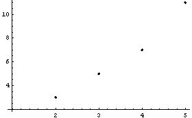
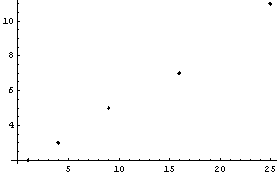
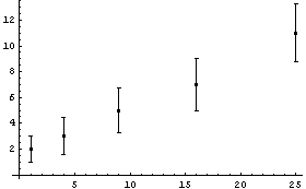
The built-in Mathematica function ListPlot is convenient for displaying data sets of one or two variables. EDA supplies a generalized version, EDAListPlot, that recognizes the EDA data format and automatically displays error bars when the data contain experimental errors. We then generate four data sets of numbers and illustrate the following (note that we "recycle" the names mydata1, mydata2, mydata3, and mydata4).

In[19]:=

Out[19]=

In[20]:=

In[21]:=

Out[21]=

In[22]:=

In[23]:=

Out[23]=

In[24]:=

In[25]:=

Out[25]=

In[26]:=

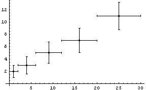
EDAListPlot has many more capabilities than those illustrated here and the full discussion of this function is found in Section 8.1.1.

As already mentioned, EDA supplies a collection of real experimental data drawn from a variety of fields of science. They are used for illustration and are located in the EDA`Data` directory, which also contains a file named Index.txt that correlates the data files with the notebooks that discuss them.

All of the data files are Mathematica packages with the exception of Aptec.txt and Cs137.dat, which are an ASCII data dump and a binary data file, respectively.

For the data files that are Mathematica packages, the data may be loaded with the EDA function LoadData.

In[27]:=

As indicated in the usage message, we can get a list of valid arguments to the program by calling it with no arguments.

In[28]:=

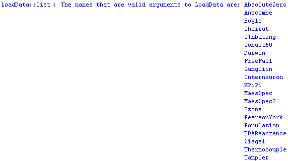
As also indicated in its usage message, LoadData has an option to control its behavior. Some functions, such as UnpackData, do not have options.

In[29]:=

Out[29]=

Other functions have many options.

In[30]:=

Out[30]//TableForm=

LoadData has a single option.

In[31]:=

Out[31]=

The option has its own usage message.

In[32]:=

As indicated, by default LoadData names the data set(s) it is loading.

In[33]:=

The option can stop the naming of the data set.

In[34]:=

Note that in all programs in Mathematica, options must be given last.

The names of the data sets, such as BoyleData, are known to the Mathematica kernel through the initialization of EDA. As discussed in Section 1.1.2, this means that you can load the data just by naming it; you may append a semicolon to the command to keep the data from being printed on your screen. You can also cause a data set to load by naming the data set in a call to a program.

In[35]:=

Out[35]=

You may prefer to use LoadData, however, because it provides error checking.

In[36]:=

Out[36]=

1.3.1 Contents of the EDA`Data` Directory

This listing does not include the files Aptec.txt or Cs137.dat, an ASCII data file and a binary data file, respectively.

In[37]:=

In[38]:=

In[39]:=

In[40]:=

In[41]:=

In[42]:=

In[43]:=

In[44]:=

In[45]:=

In[46]:=

In[47]:=

In[48]:=

In[49]:=

In[50]:=

In[51]:=

In[52]:=

In[53]:=

So far, we have loaded the data sets and then used ? to display information on the data. For the remainder of this section, we use the fact that ? will load the data automatically, as discussed in Section 1.1.2. The symbol ? is shorthand for NullInformation[ ..., LongForm False].

In[54]:=

In[55]:=

In[56]:=

In[57]:=

In[58]:=

In[59]:=

In[60]:=

In[61]:=

In[62]:=

In[63]:=

In[64]:=

In[65]:=