|
Chapter 2
Importing and Exporting Data
Often we have data on a disk and want to read it into Mathematica. The data can be either in an ASCII representation or in a binary format. This chapter discusses techniques to read such data files.
In addition to a discussion of using built-in Mathematica commands to handle these tasks, Sections 2.1 and 2.2 also introduce some EDA functions specifically designed to import and export data in ASCII files.
Section 2.3 discusses reading binary data files and Section 2.4 discusses ways to get a scanned plot of data into Mathematica.
2.1 Importing Data from an ASCII File
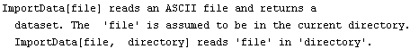
Most existing data acquisition software is capable of producing a file containing an ASCII representation of a data set. This section discusses techniques to read such a file into Mathematica, and introduces the ImportData function that often contains only the options needed to read such a file.
The first subsection is an introduction to the ImportData function, and also discusses using the built-in command ReadList function to read a data file.
The next subsection illustrates the use of ImportData using a real-world example.
The final subsection summarizes the ImportData function.
2.1.1 Introduction
Suppose we have a file named data. (Note: The examples in this section assume the existence of a file data in your current working directory. This file is not actually provided with EDA. Thus, input commands of this section are illustrative and will not actually work unless you have the specified data files.)
In[1]:=!!data
1
2
3
4
5
6
7
8
We can read the file with the built-in ReadList command.
In[2]:=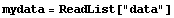
Out[2]=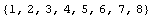
Many built-in Mathematica functions, and all those in Experimental Data Analyst, will treat this as a set of eight values of the dependent variable.
The ImportData program that is included in EDA can also read this file.
In[3]:=
In[4]:=
Out[4]=
Say instead that data has two columns of numbers.
In[5]:=!!data
1.23 2.45
4.56 17.54
5.67 26.45
We read the file with ReadList.
In[6]:=
Out[6]=
What has happened is that ReadList has interpreted each line of the file as a multiplication of two numbers, which Mathematica has evaluated. This can be suppressed by telling ReadList to read numbers.
In[7]:=
Out[7]=
If the numbers in the file represent {x, y} pairs, we can have ReadList handle each line separately by setting RecordLists to True.
In[8]:=
Out[8]=
This is just the format expected by many Mathematica functions such as Fit and ListPlot and by Experimental Data Analyst.
ImportData handles this case automatically.
In[9]:=
Out[9]=
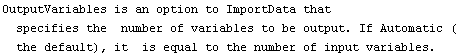
To have ImportData treat each number in the file as a value for the dependent variable, we can use the OutputVariables option.
In[10]:=
Out[10]=
We can tell ImportData to treat the numbers as a succession of {x, { y, erry}} values.
In[11]:=
Out[11]=
Imagine the file contains three numbers per line.
In[12]:=!!data
1 2 .5
3 4 .6
5 6 .7
7 8 .8
By default, ImportData will treat each line as a data point, and since there are three values for each point, it will assume that they are {x, {y, erry}} values.
In[13]:=
Out[13]=
If the final number in each line is the error associated with the first number, then the UseVariables option can be used.
In[14]:=
Out[14]=
The UseVariables option can also be used to select only some of the numbers on each line.
In[15]:=
Out[15]=
Since we have extracted two numbers per record, ImportData assumes they are {x, y} pairs. We can tell the program that the assumption is wrong.
In[16]:=
Out[16]=
Now each data point consists of {{x, errx}, {y, erry}} values.
Sometimes a data file is not "flat".
In[17]:=!!data
1 2
3
4
5 6 7 8
We can tell ImportData to treat the numbers as pairs.
In[18]:=
Out[18]=
We can extract the first of each pair.
In[19]:=
Out[19]=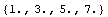
We can then put these numbers into {x, y} pairs.
In[20]:=
Out[20]=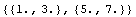
By default, ImportData assumes that either spaces or tabs separate the numbers in each row. If this is not a correct assumption, as in a data file that uses commas to separate the numbers, we can use the WordSeparators option.
In[21]:=!!data
1.2, 2.3e17
2.4, .7
12353E-2, 15
In[22]:=
Out[22]=
Of course, the other options to ImportData can be used also.
In[23]:=
Out[23]=
Sometimes a data file is not all numbers.
In[24]:=!!data
charley 17.1
joe 8
peter 42
sam 17.2
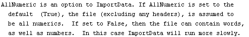
To extract the numbers from this with ReadList would require ReadList["data", Word], extracting the numeric parts which will be represented as strings, and converting the strings to numbers. ImportData provides an AllNumeric option which, if set to False, does all this automatically.
In[25]:=
Out[25]=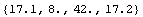
This has the correct numeric types.
In[26]:=
Out[26]=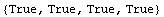
Our final introductory data set contains a header and a trailer.
In[27]:=!!data
Header for this data set.
x y erry
--------
1 2 .5
3 4 .6
5 6 .7
7 8 .8
--------
This data was taken by the
analog-analog converter at
the University of Toronto.
There are four lines of header that include one blank line and four lines of trailer information after the data.
We can still use ReadList, but we need to skip the header and tell it to read only 12 numbers.
In[28]:=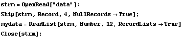
Out[30]=
The NullRecords option to Skip causes it to count the blank lines; without it the first line of data would have been lost and ReadList would have tried to read the first line of the trailer. The Close at the end is good practice to avoid having too many open files at once.
Note that to use this data for analysis, some further partitioning may be necessary.
ImportData can read the same file.
In[32]:=
Out[32]=
Of course, the other options to ImportData can be used to massage the output format.
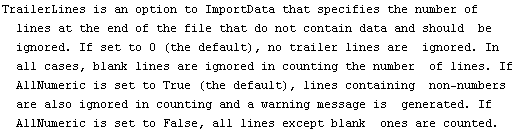
Another way to use ImportData to handle this file is to use the TrailerLines option. Since the trailer contains nonnumerics, and the trailer lines are removed after the data has been read using ReadList, we must set AllNumeric to False.
In[33]:=
Out[33]=
The formatting of the data into {x,{y, erry}} triples can be suppressed.
In[34]:=
Out[34]=
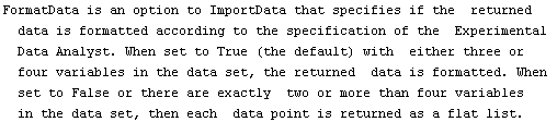
This returns each data point as a flat list of numbers. The FormatData option only has an effect for data sets with three or four variables.
Sometimes the data set has more than four variables.
In[35]:=!!data
1 2 3 4 5 6
11 12 13 14 15 16
21 22 23 24 25 26
31 32 33 34 35 36
Then ImportData returns a flat list.
In[36]:=
Out[36]=
2.1.2 A Real-World Example
Aptec Engineering, Inc. manufactures analog-digital converters and software that turns a standard PC into a nuclear multichannel analyzer. A spectrum was taken with the analyzer and saved as an ASCII print file called orig.dat.
In this example, Mathematica was running on a Hewlett-Packard UNIX computer, and the PC was on the ether network using Sun Microsystems' PC-NFS. The orig.dat file was saved on the Hewlett-Packard disk in the area that PC-NFS treats as a local DOS disk. Most UNIX platforms offer a program to convert files from DOS to UNIX; on the Hewlett-Packard machine, it is called dos2ux and was run under UNIX.
$ dos2ux orig.dat > Aptec.txt
Note that this Aptec.txt file is shipped as part of EDA and is in the Data subdirectory. To make use of this data file, you need to set the current directory to this Data subdirectory. This can be accomplished using the command SetDirectory[directory name].
Here is a summary of the file.
In[37]:=!!Aptec.txt
Aptec PC/MCA - HPS Show June 30-July 3
Aug/4/1994 12:03:47
******** 65 lines eomitted from the header listing *********
Channel Energy MeV Counts
------- ------------- ---------- ---------- ---------- ---------- ----------
0 -0.07 0 0 0 0 0
5 -0.06 0 0 0 0 0
10 -0.05 0 0 0 0 0
15 -0.04 0 0 0 0 0
20 -0.03 0 0 0 0 0
25 -0.02 0 0 0 0 0
30 -0.01 0 0 0 0 0
35 -0.01 0 0 0 3 0
40 0.00 0 0 2038 4175 3668
45 0.01 3560 3566 3593 3452 3397
50 0.02 3321 3291 3386 3155 3173
******** 801 lines eomitted from the data listing *************
4060 47.65 0 0 0 0 0
4065 48.00 0 0 0 0 0
4070 48.35 0 0 0 0 0
4075 48.69 0 0 0 0 0
4080 49.05 0 0 0 0 0
4085 49.40 0 0 0 0 0
4090 49.75 1 0 0 0 0
4095 50.11 0
Note that in the display, we have omitted a number of lines in the header and from the data. Also note that each line of data consists of seven numbers, of which columns 3, 4, 5, 6, and 7 are the counts. Finally, the last line of data contains fewer numbers than the others; by default ImportData pads the last line with zeros, which is reasonable in this case.
We read the counts from the file.
In[38]:=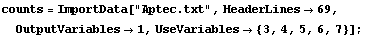

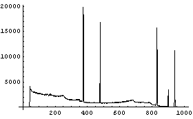
We can examine the result using Short and EDAListPlot.
In[39]:=
Out[39]//Short=
In[40]:=
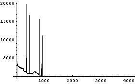
We see that the region for channels above 1000 is not of great interest.
We can extract the first 1000 counts.
In[41]:=
We can also use ImportData to read the file again to get the first 1000 counts, which is the first 200 lines. Recall that each line contains 7 numbers of which we will use only the last 5.
In[42]:=
In[43]:=
We extract the channel/energy data.
In[44]:=

Rather than make an assumption about the functional relationship between channel and energy, we can simply form an interpolation.
In[45]:=
The energy versus channel plot is interesting.
In[46]:=
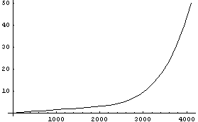
Evidently the analog-digital converter and/or counter is highly nonlinear at the higher channels, although quite linear for the first 1000 or so.
We then evaluate for the first 1000 channels.
In[47]:=
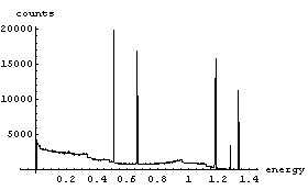
Finally, we can form a list of {energy, counts} pairs.
In[48]:=
In[49]:=
2.1.3 Summary of ImportData
This section provides a summary of the ImportData function. First, it lists the usage message for the function and all its options. Then it sketches how the function works, and in particular the order in which the options are processed.
In[50]:=
In[51]:=
Out[51]//TableForm=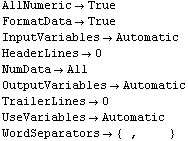
In[52]:=
In[53]:=
In[54]:=
In[55]:=
In[56]:=

In[57]:=
In[58]:=
In[59]:=

In[60]:=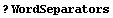

Finally, here is the order in which ImportData processes options.
1. If WordSeparators is not set to the default of {" ", "\t"}, then the AllNumeric option is set to False. This change is necessary, but it does slow down ImportData somewhat.
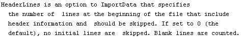
2. HeaderLines, if any, are skipped using Skip.
3. ImportData uses the built-in command ReadList, with the RecordLists option set to True. If the AllNumeric option is set to True (the default) it uses type Real; otherwise it uses type Word. If the NumData option is All (the default) it reads until the end of file; otherwise it reads NumData objects.
4. TrailerLines is set to a number, than that number of lines is then dropped from the end of the data. Note that blank lines are not counted, since ReadList has not set NullRecords to True.
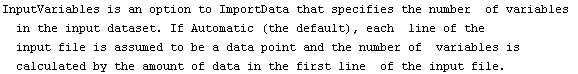
5. InputVariables is set to a number, the data is then formatted into records of InputVariables numbers each.
6. The last line of the data is padded if necessary so it has the same number of variables as the first line.
7. If UseVariables is not All, fields specified by it are then extracted, forming records of length Length[UseVariables].
8. If OutputVariables is not Automatic, the data is then formatted into records of length equal to its value.
9. If the AllNumeric option is not set to True, the fields, currently represented as strings, are converted to numbers.
10. Unless FormatData is set to False, the data is formatted into the standard form expected by Experimental Data Analyst.
2.2 Exporting Data to an ASCII File
In this section we discuss techniques to create a file containing an ASCII representation of a data set.
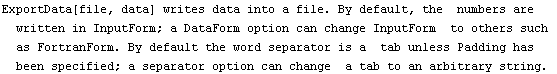
The first subsection introduces the EDA function ExportData and also discusses the built-in functions Write and WriteString.
The final subsection summarizes the ExportData function.
2.2.1 Introduction
Imagine we have a Mathematica data set.
In[1]:=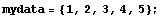
The set, including its name, can be saved into a file using the Mathematica command Save.
In[2]:=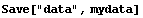
We can examine the contents of the file.
In[3]:=!!data
mydata = {1, 2, 3, 4, 5}
Warning: if the file data already exists in the current directory, the Save command will append the definition to it. Also, some versions of the front end interface have the current directory set to a system area of the disk by default, which may not be where you wish to save your work files. You can determine your current directory with the Directory command. To change where your work files are saved, you can specify an absolute pathname for data or else reset the current directory with SetDirectory.
We remove mydata from the Mathematica session.
In[4]:=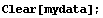
Now we can read the file back in to redefine mydata.
In[5]:=
In[6]:=
Out[6]=
The Mathematica command Write allows us to save the contents of mydata without the associated variable name.
In[7]:=
In[8]:=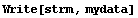
In[9]:=
In[10]:=!!data
{1, 2, 3, 4, 5}
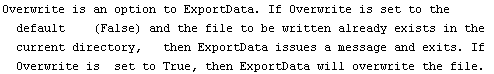
Warning: If the file data already exists in the current directory OpenWrite will truncate it to size zero. The EDA function ExportData, introduced later in this section, will not overwrite an existing file unless the defaults to the function are changed.
If we wish the file to contain five rows, each containing one of the data, we can still use Write.
In[11]:=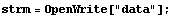
In[12]:=
In[13]:=
In[14]:=!!data
1
2
3
4
5
The built-in WriteString is more low-level than Write and can achieve the same effect.
In[15]:=
In[16]:=
In[17]:=
In[18]:=!!data
1
2
3
4
5
ExportData handles this operation automatically. First, we delete the file data we have created above.
In[19]:=
Now we write mydata into data using ExportData.
In[20]:=
In[21]:=
In[22]:=!!data
1
2
3
4
5
Internally, ExportData uses WriteString.
Below we will be illustrating the use of ExportData, always writing into a file named data. By default, ExportData will not overwrite an existing file. An option Overwrite to ExportData, if set to True, will allow ExportData to overwrite existing files. Thus, we could have all calls to ExportData below include the option.

This is certainly safe, but for our purposes we will use SetOptions to change the behavior of ExportData for the remainder of this session.
In[23]:=
Say the data contains {x, y} pairs.
In[24]:=
Out[24]=
ExportData handles this case also.
In[25]:=
In[26]:=!!data
1.234 0.000034
11.2 6.5999999999999995*^-6
21.2 0.0901
Note that in the file the columns are separated by tabs and that the second number in the second row is represented in a form that Mathematica recognizes, but that some other programs may not.
We can change the separator between columns to, say, a comma followed by a space.
In[27]:=
In[28]:=!!data
1.234, 0.000034
11.2, 6.5999999999999995*^-6
21.2, 0.0901
We can change the numbers to a form that Fortran and C can recognize.
In[29]:=
In[30]:=!!data
1.234 0.000034
11.2 6.5999999999999995e-6
21.2 0.0901
Of course, the options can be combined.
In[31]:=
In[32]:=!!data
1.234,0.000034
11.2,6.5999999999999995e-6
21.2,0.0901
Finally, the data set can contain { x, {y, erry}} values.
In[33]:=
Out[33]=
In[34]:=
In[35]:=!!data
-0.12 6.9999 6.888
1 21 321
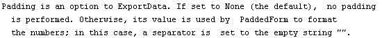
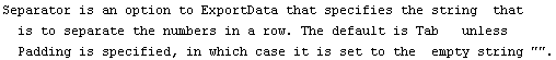
Note that because of the representation of the numbers in the first row, this may not be what you need. Specifying a Padding option causes the function to use PaddedForm with the value of the option as its second argument.
In[36]:=
This produces a file that could be read easily by a Fortran program.
In[37]:=!!data
-0.120 7.000 6.888
1.000 21.000 321.000
For the Fortran aficionado, Section 7.3 of W.T. Shaw and J. Tigg, Applied Mathematica: Getting Started, Getting It Done (Addison-Wesley, 1994) contains many helpful ideas.
2.2.2 Summary of ExportData
In[38]:=
In[39]:=

In[40]:=
In[41]:=
In[42]:=
2.3 Importing Data from a Binary File
Often data-acquisition software can produce a file containing a binary representation of a data set. Built-in Mathematica commands can be used to read such a file, with some effort. In addition, the Utilities`BinaryFiles` package, which is standard with Mathematica, automatically sets the relevant options suited to reading binary files. Finally, a MathLink version of the routines from Utilities`BinaryFiles` has been written, with the same semantics but with a very large increase in speed; as a convenience, you will find source code and/or binary versions for these routines in the FastBinaryFiles directory.
We will illustrate using the Utilities`BinaryFile` package. For further information on the routines in the package, see the documentation.
Reference: Mathematica 4.0 Standard Add-On Packages (Wolfram Research, Inc.).
Documentation on the MathLink versions of these routines may be found in the FastBinaryFiles directory.
The data file we will use is a nuclear Cesium-137 gamma-ray spectrum taken with a NaI scintillation counter. The data acquisition was performed by Version 3.07b of APTEC PCMCA/WIN software and hardware operating on an Intel-based personal computer running Windows.
Below we will be using some details about the format of the binary file that were dug out of the manual provided by APTEC.
The actual binary data file is included with EDA as the file Cs137.dat in the Data subdirectory of the EDA directory.
First we load the BinaryFiles package.
In[1]:=
Below we will be using the functions ReadBinary and ReadListBinary. Internally, ReadListBinary uses ReadBinary. The ReadBinary function from the Utilities`BinaryFiles` package has set an option.
In[2]:=
Out[2]=
This does not match the format of the data file. Rather than having to remember to set ByteOrder to LeastSignificantByteFirst each time we read a number from the file, we will set it once and for all for this Mathematica session.
In[3]:=
Out[3]=
To make use of the Cs137.dat data file, you need to set the current directory to the EDA Data subdirectory. This can be accomplished using the command SetDirectory[directory name]. Now we open the file, saving the InputStream object as str.
In[4]:=
Out[4]=
The first ten bytes of the file are the version identification string. We read them.
In[5]:=
Out[5]=
The numbers are the integer codes corresponding to the characters in the string. We can convert to characters.
In[6]:=
Out[6]=
When we opened the file, we were at the beginning of the stream. On most computer systems, our current position in the stream can be found.
In[7]:=
Out[7]=
Thus, the next ReadBinary call would start at the 11th byte.
In the file, the two bytes starting at position 14 identify the number of data points in the spectrum. We read the number.
In[8]:=
Out[8]=
In[9]:=
Out[9]=
The length of the header in the file is 1024 bytes, which is followed by the 4096 numbers corresponding to the counts. The numbers are 32-bit signed integers. So first we position the stream at the beginning of the numbers.
In[10]:=
Out[10]=
Next we read the 4096 numbers.
In[11]:=
We have two comments to make about the above command.
First, on a fast GNU/Linux workstation the command to read this fairly small file took over 5 seconds to execute; on slower hardware it will take even longer. For greater speed with large data files you may wish to use the MathLink version of ReadListBinary.
Second, ReadListBinary has set an attribute of HoldRest, which means that all but the first argument to the function are maintained in an unevaluated form. Thus, we must evaluate the value of numChannels, 4096, before passing it to ReadListBinary. Equivalently, we could have given the number 4096 directly to ReadListBinary.

Now that we have finished reading the data, we close the InputStream.
In[12]:=
Out[12]=
We can examine the data we have read.
In[13]:=
In[14]:=
Of course, if you were going to be reading a lot of binary data files produced by the APTEC software, you would probably want to write a small procedure.
ReadAptec[file_]:=Module[
{answer,numChannels,str},
SetOptions[ReadBinary,ByteOrder LeastSignificantByteFirst]; LeastSignificantByteFirst];
str=OpenReadBinary[file];
SetStreamPosition[str,14];
numChannels=ReadBinary[str,Int16];
SetStreamPosition[str,1024];
answer=ReadListBinary[str,SignedInt32,Evaluate[numChannels]];
Close[str];
answer]
This could be used directly.
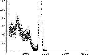
 2.4 Getting Data from a Scanned Plot
Sometimes we wish to analyze data taken by somebody else, such as might be found in a journal or book. However, many times only a graph of the data is printed. If the highest precision is required, then one must usually write to the original source and request the actual numbers. Often, however, approximate numbers that are directly available from the plot are close enough.
Provided you have access to a scanner, the Mathematica front end provides capabilities to extract those numbers, and this section is a tutorial in using that capability. The format of the scan file that can be recognized by the front end is dependent on the computer on which it is running; consult the documentation for your front end for further information. In addition, we will be using the front end's ability to select points in a graphic and to cut-and-paste the coordinates into an input cell; again, the exact details of how to do this will depend on the computer being used.
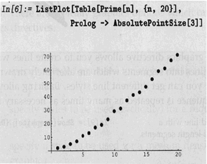
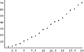
We will use as an example a plot whose result is known: a plot generated by ListPlot that appears on page 487 of Stephen Wolfram's The Mathematica Book, 4th edition (Wolfram Media and Cambridge Univ. Press, 1999). After scanning the relevant page from the book, we will import it into the notebook.
Some details: this notebook was written on a UNIX workstation and the file format recognized by this version of the front end is GIF. This GIF has been converted by the front end to PostScript, so that it is readable on all hardware platforms. Also, the scan has been reduced to fit in the standard-sized window above. The numbers below were generated with the full-size original scan, which gives the best precision. Nonetheless, you may use the graphic above to generate numbers equivalent to those below; the modifications to the graphic means that the actual values will be different.
We will first locate the graphics coordinates of the x axis at zero and 20. The actual numbers were generated by cutting and pasting from the graphic; everything else was typed in by hand.
In[1]:=
In[2]:=
The conversion from graphics coordinates to the actual units of the x axis is linear.
 Now we evaluate the numbers.
In[3]:=
Out[3]=
In[4]:=
Out[4]=
We similarly convert graphics coordinates to the units of the y axis.
In[5]:=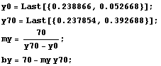
Finally, we extract the coordinates of the data points.
In[9]:=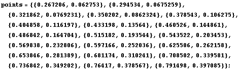
Then the x values, converted to the units of the plot, can be calculated.
In[10]:=
Out[10]=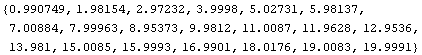
This compares well with the actual integers 1, 2, ... , 19, 20.
We similarly find the y values.
In[11]:=
Out[11]=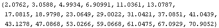
These are within a few percent of the actual numbers.
In[12]:=
Out[12]=
We plot the scanned data results.
In[13]:=
In[14]:=
|