|
Chapter 7
Robust Fitting
In this chapter we discuss ways to circumvent a problem that was discussed in Chapter 4: least-squares techniques are not resistant to a wild data point. Such wild data points are often called "outliers." The "robust" fitters discussed here avoid that weakness of least-squares techniques. One price that is paid, however, is that explicit errors in the data are ignored, and no truly meaningful estimates of errors in the fitted parameters are possible. Also, these techniques are slower than conventional methods.
There is also a serious danger in these techniques. They assume that the model, either a line or a curve, is correct for the data and any data points that are not consistent with the model are suppressed. Very few scientific advances would occur if researchers always suppressed data that does not match preconceived expectations. The topic of suppressing or rejecting measurements is also discussed in Section 3.2.4.
The discussion below assumes some familiarity with the concepts and syntax discussed in Chapter 4. The LinearFit function introduced in that chapter should usually be tried before using the techniques discussed here.
7.1 Introduction
7.1.1 Using the Median
As has been mentioned many times, the mean or average is not resistant to a wild data point, which will badly distort the result of the calculation. It is in exactly this sense that least-squares techniques in general are not resistant.
We have also mentioned numerous times that the median is resistant to a wild datum — that is, it is "robust" — and that fact is used in the RobustLineFit function introduced in this subsection. The central idea is that the routine divides the data into three groups based on the value of the independent variable. Then the medians of the independent and dependent variables are calculated for each group, and a straight-line fit is made to these medians.
We first load and display some data on radioactive dating.
In[1]:=
In[2]:=

In[3]:=

In[4]:=
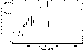
Further information on this data appears in Chapter 8.
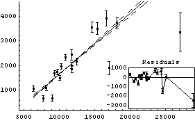
If the thorium and carbon-14 dating agreed, the dependent variable should be zero within errors, which is clearly not the case. We fit the data to a straight line using the EDA function LinearFit.
In[5]:=
Out[5]=
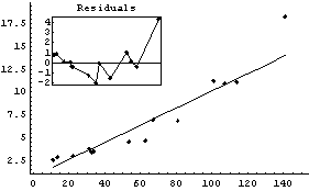
In this fit the two "outliers" in the data are having a marked effect on the results of the fit, as can be seen in the plots.
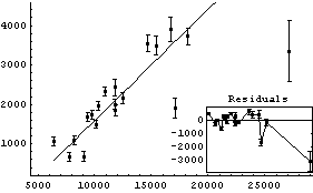
We do a robust straight-line fit to the data using RobustLineFit.
In[6]:=
Out[6]=
Note that the function requires a parameter name in its input, just like LinearFit, and by default returns rules for array members of that parameter, again just like LinearFit.
As discussed in Section 7.2, for this technique the concept of degrees of freedom has no meaning. Nonetheless, the function does return a ChiSquared using the errors in the experimental data as the weights. As we shall see, if the data has no explicit errors, a SumOfSquares is returned. In both cases, interpreting this number is indirect.
We examine the data.
In[7]:=
Out[7]=
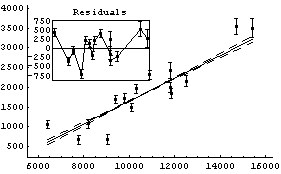
This shows that the two "wild" data points are at the end and the fourth from the end. We form a new data set with these two points dropped.
In[8]:=
Fitting this to a straight line yields almost the same fit that we got for the full data set with RobustLineFit.
In[9]:=
Out[9]=
The advantage of RobustLineFit, however, is that in some sense it provides an "objective" estimate of whether or not a data point is wild, and does not involve explicitly throwing out any data.
As a final example using RobustLineFit, we return to the ganglion data already discussed in Chapters 4 and 6.
In[10]:=

In[11]:=
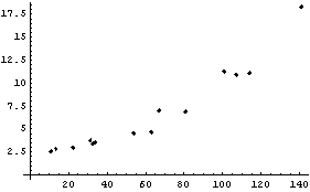
So far, we have (1) fit the data to a parabola as well as a line, (2) fit the data to a straight line with the last data point dropped, and (3) done a loess fit to the residuals of various linear fits. We now do a robust fit to a line.
In[12]:=
Out[12]=
Here again, the result gives us some indication that a straight line is not a good model for this data unless we treat the last data point as an outlier.
7.1.2 Using Weighting Techniques
Another way to do robust fitting is to realize that the data points we wish to suppress are those with high residuals. Say we have done a fit and the residuals for each data point are the following.

We form a set of weights.

First we define a cutoff.

Values of the dependent value greater than this cutoff are set to zero. For values smaller than the cutoff, the weights are "bi-square" weights of the residuals. For example, if the cutoff is 15 the weights look like this.
In[13]:=
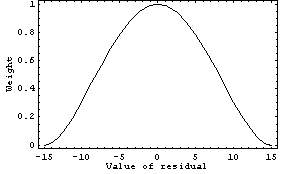
A brief technical note: Because we are going to convert these weights to errors below by taking the reciprocal of them, the minimum value of a weight cannot be exactly zero. Instead these weights are set to the minimum positive number that can be used on a particular computer, $MinMachineNumber.
The weights are converted to effective errors in the dependent variable.

Then the fit is iterated until it converges.
This is exactly the technique used by RobustCurveFit.
In[16]:=
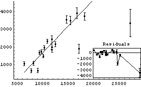
Out[16]=
Note that the input arguments to RobustCurveFit are identical to those of the EDA function LinearFit. LinearFit is actually used internally by RobustCurveFit.
The PseudoChiSquared returned by the routine is the chi-squared statistic calculated assuming that the errors in the dependent variable generated by the bi-square weights are the correct errors. Thus, its interpretation is indirect.
The DegreesOfFreedom returned is the number of data points minus the number of parameters to which we are fitting (the standard definition) minus the number of data points whose weights are set to zero.
If the model matches the data reasonably well, then RobustCurveFit should produce a fit with little or no difference from LinearFit. Using the ganglion data once more illustrates this.
In[17]:=
Out[17]=
In[18]:=
Out[18]=
Note that we could not have used RobustLineFit for this, since it is only capable of fitting to straight lines.
Finally, RobustCurveFit can be used as a robust averager of data. For example, the following command generates 20 data points fairly close to 1.5 and a single data point equal to 100.
In[19]:=
We use the Mean and Median functions from the standard Statistics`DescriptiveStatistics` package on this data.
In[22]:=
In[23]:=
Out[23]=
In[24]:=
Out[24]=
We can also examine the data with the EDA function EDAHistogram; this function is discussed further in Chapter 8.
In[25]:=
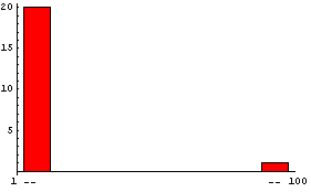
Fitting this data to a polynomial with powers of {0} means we have forced the slope and all other terms involving the independent variable to zero. Thus, a[0] should be the mean.
In[26]:=
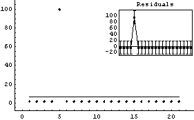
Out[26]=
This result shows clearly that the least-square technique used by LinearFit is not robust and the answer is exactly the same as produced above by Mean. However, using RobustCurveFit gives a robust answer.
In[27]:=
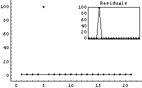
Out[27]=
In fact, this result is almost exactly the average of all the numbers except the one outlier.
In[28]:=
Out[28]=
The result of RobustCurveFit is also within 0.3% of the median of the full data set.
7.2 Details
In[1]:=
7.2.1 RobustCurveFit
The algorithm used by RobustCurveFit is described in Section 7.1.2. The function has the following options.
In[2]:=
Out[2]//TableForm=
The LinearFit function discussed in Chapter 4 has these same options with the same meanings.
Experience has shown that a MaximumIterations of 5 should almost always be sufficient for RobustCurveFit, but the option allows the number to be increased if necessary.
The ReturnErrors option, if set to True, causes the routine to attempt to estimate and return errors in the fitted parameters.
In[3]:=
Out[3]=
However, these numbers should be taken with a "grain of salt" since the errors in the dependent variable are fakes: they are generated from the bi-square weighted residuals.
Nonetheless, to have these errors in the fit parameters adjust the significant figures in the answer, the UseSignificantFigures option may be used.
In[4]:=
Out[4]=
To have RobustCurveFit return a function of an independent variable, say c14, instead of a list of rules, the ReturnFunction option may be used.
In[5]:=
Out[5]=
The EDAShowProgress option enables monitoring of the progress of the function.
In[6]:=


Out[6]=
Finally, as already seen in the examples above, setting ShowFit to False suppresses the graph of the results. This last example has stored the fit parameters in result. The graph can be generated at a later time with the EDA function ShowLinearFit, which is discussed in Section 4.5.2.
In[7]:=

An extensive discussion of the bi-square weighting method used by RobustCurveFit can be found in Cleveland.
Reference: William S. Cleveland, Visualizing Data (AT&T Bell Laboratories, 1993), passim.
7.2.2 RobustLineFit
As mentioned in Section 7.1.1, the central ideal of RobustLineFit is that it divides the data into three groups based on the value of the independent variable. We will call these groups Left, Middle, and Right, respectively. Then the medians of the independent and dependent variables are calculated for each of the three groups, and a straight line is fit to the medians.
The three-group median method implemented by RobustLineFit is derived from Tukey, although in its original form the algorithm is not always stable. Thus, here we use a modification with greatly improved stability due to Johnstone and Velleman.
References:
John W. Tukey, Exploratory Data Analysis (John Wiley, 1970).
I. Johnstone and P.F.Velleman, 1981 Proc. Statistical Computation Section, American Statistics Assoc. (1982), p. 218.
RobustLineFit has the following options.
In[8]:=
Out[8]//TableForm=
All of these options except Groups have identical meanings to the same options for LinearFit and RobustCurveFit. We will discuss Groups in a moment.
Experience has shown that a MaximumIterations of 5 is almost always sufficient, although the option allows it to be increased if necessary.
When ReturnFunction is set to True, the routine returns a function of the independent variable parameter, instead of a set of rules for a parameter.
Setting ShowFit to False suppresses the display of the results of the fit. The EDA function ShowLinearFit can later display the result from RobustLineFit.
As usual, EDAShowProgress gives information about the progress of the fit. Below are some examples using this option.
The Groups option controls how the data are divided into three groups. When it is set to Automatic, the groups are as close as possible to having the same number of data points in them. However, no two groups are allowed to have the same value of the independent variable in them, so some shifting is necessary. The following example illustrates this shifting.
In[9]:=
Out[10]=
In[11]:=


Out[11]=
Although it tries to be smart about forming groups, occasionally RobustLineFit fails.
In[12]:=
Out[13]=
In[14]:=


Out[14]=
We can force the program to use group sizes of 2, 2, and 6, respectively.
In[15]:=


Out[15]=
Just specifying ratios of the group sizes has the same effect.
In[16]:=


Out[16]=
Note the warning message generated above. As discussed below, there is a desire for groups of about the same size.
The Left and Right groups alone are used to determine the slope of the line. Thus, there is a balance needed between having a reasonable sized group and having these two groups fairly far away from each other. Once the slope has been determined through iteration, the intercept is calculated from the residuals and the median of the independent variable of the Middle group.
There is a history of two-group and three-group median methods going back to at least 1940. A review of that history and further details of the algorithm used by RobustLineFit can be found in Emerson and Hoaglin.
Reference: John D. Emerson and David C. Hoaglin, in David C. Hoaglin, Frederick Mosteller, and John W. Tukey, eds., Understanding Robust and Exploratory Data Analysis (Wiley-Interscience, 1983), Chapter 5.
7.2.3 Comparing RobustCurveFit and RobustLineFit
When doing a robust fit to a line, RobustLineFit is much faster than RobustCurveFit. For example, below we generate some made-up data of 1000 points of which 5 are outliers.
In[17]:=
In[19]:=
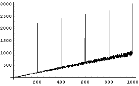
We fit to a straight line and generate timing information.
In[20]:=
Out[20]=
In[21]:=
Out[21]=
Although you probably will not get exactly the same timing numbers on your computer, you will find that RobustLineFit is much faster than RobustCurveFit for most large datasets. Considering the details described above of how the two routines work, this result is hardly surprising.
Of course, the comparative slowness of RobustCurveFit is balanced by the fact that it can fit to arbitrary polynomials.
In addition, RobustLineFit devotes most of its effort to the determination of the slope, which is usually the parameter of most interest. RobustCurveFit, on the other hand, emphasizes the slope and intercept essentially equally when fitting to a line.
7.3 Summary of the RobustFit Package
In[1]:=
In[2]:=

In[3]:=
Out[3]//TableForm=
In[4]:=

In[5]:=

In[6]:=

In[7]:=

In[8]:=

In[9]:=

In[10]:=

In[11]:=
Out[11]//TableForm=
In[12]:=

In[13]:=

In[14]:=

In[15]:=

In[16]:=

|