Smoothing Data, Filling Missing Data, and Nonparametric Fitting

Chapter 6

Smoothing Data, Filling Missing

Data, and Nonparametric Fitting

Here we discuss dangerous techniques: smoothing data to eliminate noise and filling in missing data values. The reason for the danger is that any such method assumes that the data does not contain small-scale structure, although often nothing supports the assumption except the analyst's hunch or hope.

This chapter also discusses fitting data when a model is either not available or not desired: this is called "nonparametric" fitting.

6.1 Introduction

6.1.1 Smoothing with Averaging Techniques

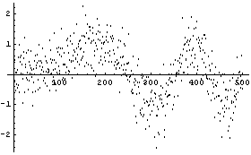
Often one is confronted with "noisy" data. For example, here is a "chirp" signal.

In[1]:=

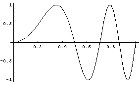
The signal is so named because it resembles the chirp of a bird.

Perhaps the signal has noise.

In[2]:=

In[3]:=

In[4]:=

In[5]:=

Here the noise is a randomized Gaussian with mean of 0 and standard deviation of 0.5. In this example, we have 500 data points.

The routine that generated this data is supplied as part of the EDA`SmoothData` package.

In[6]:=

One technique to smooth the data is to take overlapping subsets of the data and average the values of each. We will illustrate with a very simple data set.

In[7]:=

The following line calculates the mean by adding up all the elements of the list and dividing by the length of the list.

In[8]:=

In[9]:=

Out[9]=

The built-in Mathematica function Partition divides its input into partitioned subsets.

In[10]:=

Out[10]=

We can find the average of each subset.

In[11]:=

Out[11]=

We apply this idea to the noisy chirp signal, with 43 points in each subset.

In[12]:=

In[13]:=

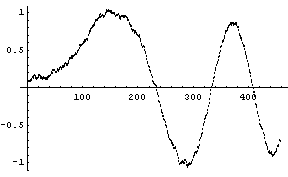
Note that this procedure ends up with less data than the input.

In[14]:=

Out[14]=

The EDA function SmoothData uses almost exactly the same method by default.

In[15]:=

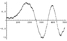
Here is the default number of points in the subsets.

points=2*Floor[Sqrt[[Length[mydata]]]]-1

For this data the number of points is equal to 43.

Near the left- and right-hand sides, SmoothData has constructed subsets of the data with fewer than points members; thus it returns the same number of data points as mydata. Of course, with fewer points the averaging at these sides will be somewhat "wilder".

The number of points can be controlled with an option.

In[16]:=

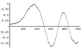
This smooths the data more than the previous example but has lost some information, particularly at the right-hand side. Note also that the program systematically decreases the amplitude of the signal at larger values of t for this data.

Points should be an odd integer less than the number of data points.

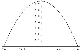
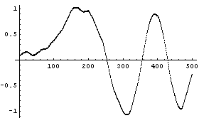
A similar method of smoothing data is based on the realization that the value at the center of each subset is more likely to be close to the actual data point than values at the ends of the subset. Thus, you can weight the values in the subset. Typically, a parabolic weight is used, normalized so the area under the curve is 1. Thus, this is what the weighting looks like.

In[17]:=

SmoothData provides an option for this type of weighting.

In[18]:=

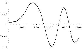
The number of points in each partition can also be adjusted.

In[19]:=

Although not an issue for this example data set, taking the average of the subset can lead to problems if the noise signal contains large variations. This is because one wild data point can seize control of an average, which will affect the result of each partition of the data in which it appears. A more robust operation than the average is the median. SmoothData can use the median.

In[20]:=

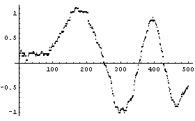
For this data, this procedure yields the least smooth of the three methods.

We construct a dataset for which there is one wild data point out of the 500 total points.

In[21]:=

The effect on the two averaging methods is large.

In[22]:=

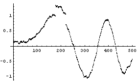
In[23]:=

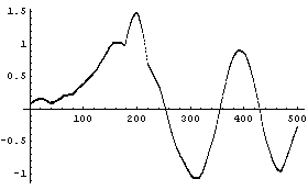
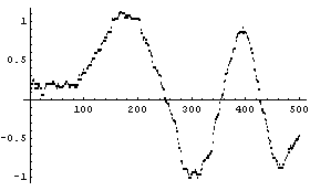
But the median is robust.

In[24]:=

Finally, imagine the chirp signal also has a small sine wave added for a region.

In[25]:=

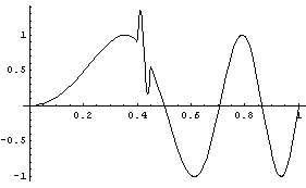
We add random noise as before, this time with a standard deviation of 0.1. As a convenience, a routine to generate test data is included named SmoothTestData. We use it to generate a data set.

In[26]:=

In[27]:=

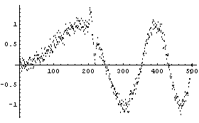
SmoothData misses the small structure almost entirely.

In[28]:=

We can reduce the number of points to preserve the structure.

In[29]:=

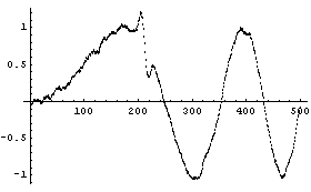
This illustrates the danger referred to at the beginning: blindly using SmoothData or any other smoothing algorithm can cause real structure in the data to be lost. As Press, et al., say, think about "letting it all hang out. (Have you considered showing the data as they actually are?)" [Numerical Recipes in C, p. 514].

6.1.2 Fourier Filters

SmoothData can use another method, based on the Fourier transform.

If, as in our examples, the signal is a function of time, then the Fourier transform of the signal is a function of the frequency. We can weight the transform to suppress the high-frequency components and then take the inverse Fourier transform to produce a filtered signal.

We use the same data as in the previous subsection and smooth it using a Fourier filter.

In[1]:=

In[2]:=

In[3]:=

In[4]:=

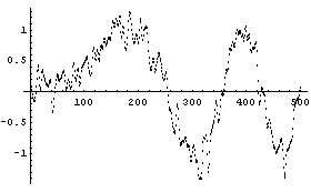
For this method, the weighting is a Gaussian centered at zero frequency. Points is the number of frequency points corresponding to the standard deviation squared of the Gaussian. Thus, as opposed to the averaging methods, decreasing the number of points increases the smoothing.

For example, the previous plot is for the default of 43 points. Here is the result for 11 points.

In[5]:=

The method is not very robust. Using the data from the previous subsection with one wild point shows that a single data point can have a large effect.

In[6]:=

In[7]:=

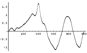
We can reduce the number of frequency points to reduce this effect.

In[8]:=

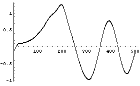
For the signal with a small sine wave added to a region, the default number of points keeps the small added term in the smoothed spectrum.

In[9]:=

In[10]:=

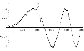
We can filter out the high-frequency signal.

In[11]:=

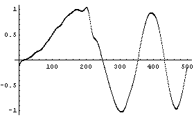
6.1.3 Loess Fitting

As hikers know, loess is a surface of loam such as is deposited by the wind. Loess fitting is similar to the method using WeightedAverage that can optionally be used by SmoothData, as described in Section 6.1.1. However, here we take each weighted subset of the data and fit it to either a straight line or a second- or third-order polynomial.

We loess fit the same noisy chirp signal, mydata, that we have used throughout this chapter, to a second-order polynomial.

In[1]:=

In[2]:=

In[3]:=

In[4]:=

In[5]:=

In[6]:=

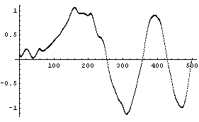
The second parameter in the call to LoessFit must be either 1, 2, or 3, giving a first-order, second-order, or third-order polynomial fit, respectively.

In addition, just as for SmoothData, the number of points in each subset may be set using the Points option, which should be set to an odd integer.

An extensive discussion of the LoessFit method appears in William S. Cleveland, Visualizing Data (AT&T Bell Laboratories, 1993). Cleveland uses a parameter alpha to choose the number of points.

points=alpha*Length[data]

LoessFit can accept an EDAAlpha option as a way of choosing the points.

In[7]:=

SmoothData[ ... , Method -> WeightedAverage] uses a parabolic weighting. LoessFit uses a tricubic weighting.

Here delta is between -1 and 1. This is what that weighting looks like.

In[8]:=

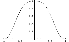
While loess fitting can be viewed as a data-smoothing technique, it can also be thought of as a fit to a data set when we cannot expect to find a parametric family, such as a straight line, to model the data. Thus it is a nonparametric fitter.

As opposed to SmoothData, LoessFit can process data with the value of Points greater than the number of data points. In this case, the weights are divided by (Points / number of data points).

Because each partition of the data set is individually fit to a line or a second- or third-order polynomial, as a data smoother LoessFit is the slowest of the techniques discussed so far in this chapter.

For example, here are some timings on a particular computer.

In[9]:=

Out[9]=

In[10]:=

Out[10]=

In[11]:=

Out[11]=

In[12]:=

Out[12]=

In[13]:=

Out[13]=

This timing is hardly surprising since LoessFit in this case performs 500 straight-line fits using the Mathematica function Fit.

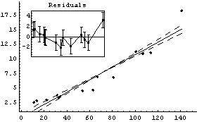
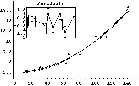
However, as a nonparametric fitter LoessFit can sometimes be very useful. For example, in Chapter 4 we were trying to decide whether some data on the ganglia of cat fetuses were best modeled by a straight line or a parabola. We repeat two fits from that chapter.

In[14]:=

Out[14]=

In[15]:=

Out[15]=

We display the residuals and a LoessFit to them for the first fit.

In[16]:=

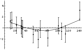
The joined points show the smoothing effect of LoessFit.

We repeat for the second fit.

In[17]:=

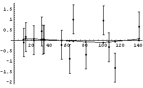
As can be seen, the residuals for this second fit are much closer to zero, and are consistent with having zero slope. This is further indication of the fact, discussed in Chapter 4, that this data appears to be better fit by a parabola than a straight line.

6.1.4 Using Mathematica Built-in Functions

The richness of Mathematica often provides just the tools needed to do a particular analysis without needing to load any packages from EDA. Here we provide a small example using some mass spectrometer data.

In[1]:=

In[2]:=

In[3]:=

In[4]:=

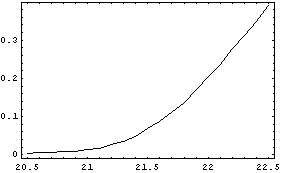
If the instrument resolution were perfect, we would expect the plot to be discontinuous. For example, if the ionization voltage were 21.5 volts, the plot would look like this.

In[5]:=

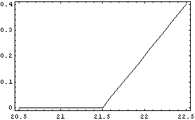
If we can approximate the experimental data as a smooth curve, we would expect the ionization voltage to be the point on the curve where the second derivative is a maximum. We can form such a smooth curve using the NumericalMath`PolynomialFit` package and fitting to a fairly high-order polynomial.

In[6]:=

Out[7]=

Note that there is no theoretical reason why we would expect that this data would be modeled by a fifth-order polynomial, except that we expect the data to be smooth. Also, the Fit routine could be used here, instead of PolynomialFit.

Examining the residuals of the fit indicates a fairly good result, since they are all numerically small compared to the values of the dependent variable.

In[8]:=

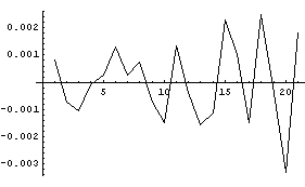
We calculate and graph the first derivative.

In[11]:=

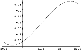
Similarly, we calculate and graph the second derivative.

In[13]:=

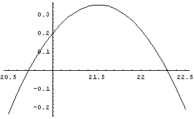
The maximum occurs when the third derivative is zero.

In[15]:=

Out[15]=

The first solution is not physical, so the ionization voltage is 21.5 volts. From the graph of the second derivatives, the size of the residuals of the original fit, and knowledge of the apparatus, the precision of this determination is estimated to be ± 0.2 volts.

6.1.5 Smoothing an Interpolation

In the previous subsection we formed a polynomial fit to find a "smooth" curve through some data, and then found the maximum in the second derivative of that curve.

Now we form and examine an interpolation of that same data.

In[1]:=

In[2]:=

In[3]:=

Out[3]=

In[4]:=

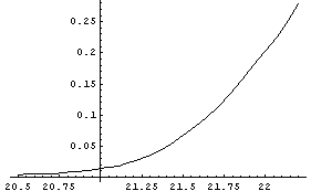
We take the derivative of the interpolation and then plot it.

In[5]:=

Out[5]=

In[6]:=

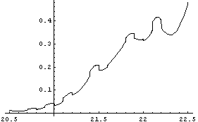
Note that the plot is not smooth. The reason is that Interpolation is constrained to go exactly through every data point. When there is a small amount of noise in the data, this constraint leads to a jagged first derivative.

The second derivative is even worse.

In[7]:=

Out[7]=

In[8]:=

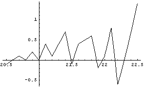
We will use the SmoothData function discussed in Section 6.1.1.1 to construct a "smoothed" table of values for the first derivative. We generate 50 points and have SmoothData smooth them in groups of 15.

In[9]:=

Out[9]=

In[10]:=

In[11]:=

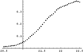
This plot looks much better.

In[12]:=

Out[12]=

We construct an interpolation of this data.

In[13]:=

Out[13]=

We take the derivative.

In[14]:=

Out[14]=

In[15]:=

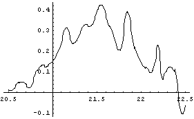
We smooth ddint.

In[16]:=

In[17]:=

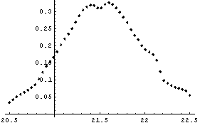
So, we conclude that the maximum in the second derivative is about 21.5 ± 0.2 volts. This is consistent with the result from the previous subsection.

Although this example does not significantly improve the result we achieved in the previous subsection using polynomial fits, the technique described here can be used for data in which no polynomial fit approximation is possible. In fact, this is the technique used by the EDA function FindPeaks described in Chapter 8.

6.1.6 Filling Missing Data

Most of EDA deals with the most common form of data encountered in science and engineering: {x, y} pairs, possibly with errors in one or both coordinates. For such "bivariate" data, finding a value for a missing data point is usually easy. If we have a model for the data, we can fit the data to the model and evaluate the fit result at the missing point; if we lack a model then the Mathematica built-in function Interpolation returns an InterpolatingFunction which can similarly be evaluated for the missing point.

If the data is a matrix of values, the EDA function FillData introduced here fills in missing values. Such a data structure is called "multivariate" since each data point in the matrix actually represents an {x, y, value} triple. We illustrate this with some data on ozone levels in the atmosphere.

In[1]:=

In[2]:=

In[3]:=

In[4]:=

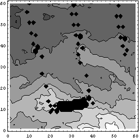
Nimbus 7 is in a south-north sun synchronous polar orbit such that it is always close to local noon/midnight beneath the satellite. The black areas in the plot are missing data; they are represented by values of 0. The small missing areas are because the width of data-taking does not completely overlap with the width of the next pass of the satellite; the larger missing area is due to a temporary failure in the down-link or perhaps a brief shutdown of the spectrometer for maintenance.

We will also be using the small made-up data sets myData1 and myData2. The latter is a 5 × 6 matrix with some structure, while the former has some missing values inserted.

In[5]:=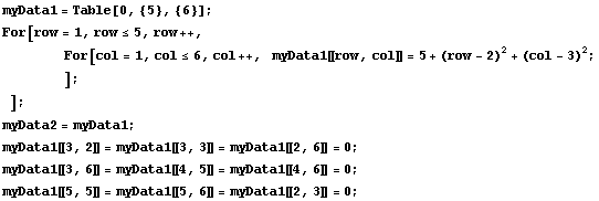

In[11]:=

Out[11]//MatrixForm=

Again, the missing values are represented by zeros, which are the black areas in the density plot.

In[12]:=

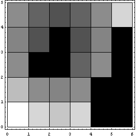
In the above plot, Reverse has been used to reverse the rows so that the display matches the printed MatrixForm.

The data set myData2 has no missing values, and a somewhat symmetric structure.

In[13]:=

Out[13]//MatrixForm=

In[14]:=

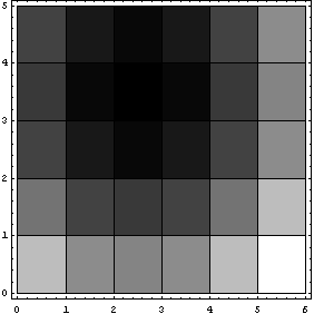
FillData can fill in missing values.

In[15]:=

In[16]:=

Out[16]//MatrixForm=

In[17]:=

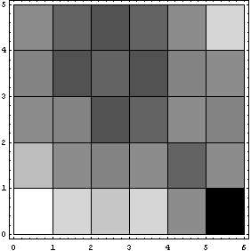
The default method for FillData, EDANearestNeighbor, is to fill the missing point with the value of a nearest adjacent neighbor. Since the point in the lower right had no non-missing neighbors, it was not filled. We can direct FillData to do two passes on the data by setting the MaximumIterations option to 2.

In[18]:=

Out[18]//MatrixForm=

Now there are no missing values.

We can similarly use FillData on OzoneData.

In[19]:=

The small missing areas are filled and the large missing area is now smaller. A second iteration fills the large area entirely.

In[20]:=

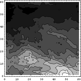
The reason the second plot above is so much darker than the first is that ListContourPlot scales from black to white based on the smallest and largest value in its input data; in the second case we have no explicit zeros. We can expand the grayscale of the second plot.

In[21]:=

If you are reading this notebook online and you are connected to a Mathematica kernel and using a color monitor, you can view the plot in color. To do this use ListDensityPlot.

You may then use the fact that the eye can distinguish about an order-of-magnitude more colors than grayscales to make it easier for you to see the structure in the ozone data.

EDANearestNeighbor, the default Method used by FillData, is the fastest and simplest available. However, other methods are available.

The second simplest method for FillData is SmoothFill, in which each missing value is filled in with the average value of all the non-missing adjacent neighbors.

In[22]:=

Out[22]//MatrixForm=

This method does a nice job on the ozone data, but it works a little more slowly than EDANearestNeighbor.

In[23]:=

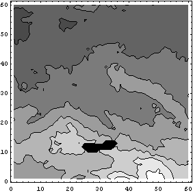
A related method reasons that if averaging is a good idea for filling in missing values, it is a better idea to average all the values in the data set.

In[24]:=

Out[24]//MatrixForm=

Although this method can sometimes be useful, it is always dangerous to actually alter any real data points. Nonetheless, this method does smooth out noise in the data. In fact, one could smooth the data down to a uniform gray by repeated iterations except that FillData never attempts to work on data that has no missing values.

The final two related methods available to FillData are RowInterpolation and ColumnInterpolation. Each uses Mathematica's Interpolation function to interpolate missing data; RowInterpolation interpolates the rows, ColumnInterpolation the columns. Note that the methods do not extrapolate to edges where there is missing data.

For myData1, nearly identical to myData2 but with added some missing values,the outputs of both RowInterpolation and ColumnInterpolation are identical and except for the missing data at the edges also duplicate the full data set.

In[25]:=

Out[25]//MatrixForm=

In[26]:=

Out[26]//MatrixForm=

In[27]:=

Out[27]//MatrixForm=

In[28]:=

Out[28]//MatrixForm=

For the ozone data, the large missing area in the center is aligned approximately horizontally. Also, the data was taken as the Nimbus satellite was moving from the south to the north, so data in the same column was taken as part of the same sweep of the satellite. Thus the data itself suggests that ColumnInterpolation is the preferred interpolation.

In[29]:=

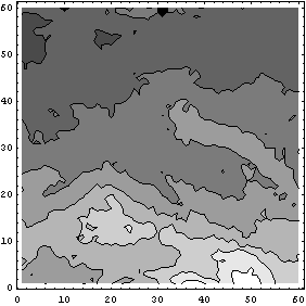
There are three missing values located at the North Pole. We can use another method in a second pass to fill them.

In[30]:=

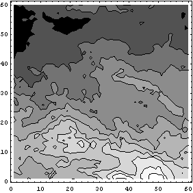
As we mentioned, ColumnInterpolation is preferred over RowInterpolation for this data, in part because of the shape of the big block of missing values. The word "big", however, means compared to the size of the structures that we see in the nonmissing parts of the data. The StructureSize option to FillData can be used by both interpolation methods and allows us to specify the size of structures in the data; FillData will not interpolate across sections of rows or columns where the number of missing values is greater than or equal to this number.

In[31]:=

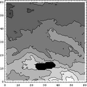
So far we have assumed that data values of zero were the missing ones. The MissingIs option allows us to choose another value.

In[32]:=

Out[32]//MatrixForm=

Here the 15 in the upper right corner has been replaced by the value of its neighbor, 10.

In[33]:=

Out[33]//MatrixForm=

Now the missing value in the upper right corner has been replaced by the mean of 10, 9, and 0.

6.1.7 References

William S. Cleveland, Visualizing Data (AT&T Bell Labs, 1993). The principles of loess fitting are discussed with clarity throughout this book

Brand Fortner, The Data Handbook (SpyGlass Inc., 1992), Chapter 11. A survey of techniques for filling missing data, many of which are used by the EDA function FillData

K.S. Riedel and A. Sidorenko, Computers in Physics 8 (1994), 402. A tutorial on the sometimes sophisticated algorithms used to smooth noise in a data set

6.2 Details

6.2.1 Nonmonotonic Data and Related Assumptions

When the dependent variable is not monotonic, the results from the EDA functions discussed in this chapter may be incorrect.

The default behavior of SmoothData, which is just a simple average, weakly assumes that the data is monotonic. This method does not handle local minima or maxima in the data very well.

The WeightedAverage method for SmoothData uses the values of the independent variable to choose the weights to multiply with the dependent variable. Thus, there is no assumption of monotonicity. This method does not handle local minima or maxima in the data very well.

The SimpleMedian method of SmoothData makes no assumption about monotonicity. This method does not handle local minima or maxima in the data very well.

The WeightedFourier method of SmoothData strongly assumes that the dependent variable is monotonic.

In[1]:=

In[2]:=

The WeightedFourier method handles local minima or maxima better than any other method available for SmoothData.

For nonmonotonic data for which smoothing with WeightedFourier is desired, it may be reasonable to use the Mathematica built-in function Interpolation on the data, and then use Table to form a data set that is monotonic in the independent variable.

LoessFit makes no assumptions about the independent variable being monotonic, since it uses the independent variable to calculate the weights to multiply with the dependent variable. Particularly for polynomial fit or order greater than 1, it also handles local minima and maxima in the data very well.

6.2.2 Comparing Various Smoothing Methods

Most of the smoothing examples in this chapter have concentrated on the "chirp" signal. Here we discuss some of the issues in selecting one of the methods available in this package.

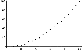
First we generate some noisy data for a parabola.

In[1]:=

In[3]:=

In[4]:=

In[5]:=

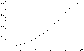
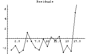
Clearly the right-hand side, where the data is beginning to increase rapidly, is pulled down from a reasonable value by this procedure. Now extract the y values from try and plot the residuals between them and the result of SmoothData.

In[6]:=

In[7]:=

Reducing the number of points in each subset used by SmoothData helps somewhat.

In[8]:=

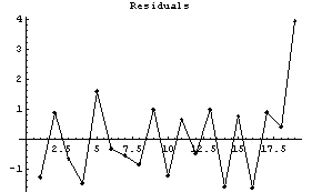
A moment's thought makes it clear that this method will always have these kinds of difficulties at any edge where the slope is significant.

We now examine the WeightedAverage method.

In[9]:=

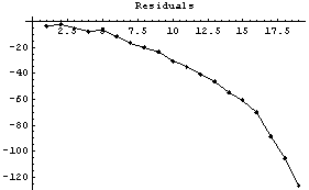
The graph shows that the method gives values much too large at the right-hand side. We reduce the number of points.

In[10]:=

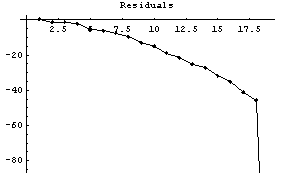
This change helps all but the very last result. Again, this behavior is a general feature of this method near an edge with a large slope.

We examine the SimpleMedian method.

In[11]:=

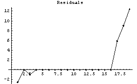
This method is also having problems at the right-hand side, and some difficulty on the left. Reducing the number of points helps for this case.

In[12]:=

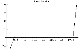
For data with a larger noise component, reducing the number of points will usually worsen the result.

Next, we look at the WeightedFourier method.

In[13]:=

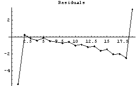
This method is having problems on both the left and right sides. The warning message is due to the details of the Fourier transform; it is discussed in Section 6.2.2.1.

Finally, we will examine LoessFit for straight line and quadratic fits.

In[14]:=

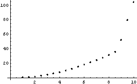
In[15]:=

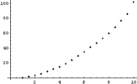
We extract and plot the residuals.

In[16]:=

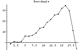
In[17]:=

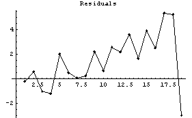
Notice that the values of the residuals are much smaller for the higher-order polynomial fit.

6.2.2.1 More on the WeightedFourier Method

In the previous section, the WeightedFourier method of SmoothData generated a warning message.

SmoothData::bigsigma: Warning: the standard deviation of the weight function is very large.

Here we discuss what the message meant.

Because the data sets we are dealing with are collections of discrete points, the Fourier transform of the data will show "aliases" or "Nyquist pairs". We will illustrate with a sampled sine wave.

In[18]:=

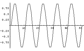
We graph the Fourier transform.

In[19]:=

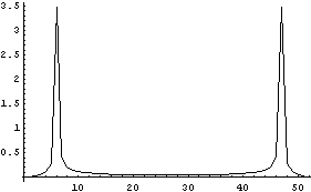
The WeightedFourier method of SmoothData weights the transform with a Gaussian, and due to these aliases, it actually weights both sides. So, for a standard deviation sigma of 5, the weighting can be graphed.

In[20]:=

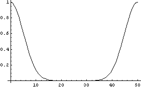
If Points is large, these two Gaussians can overlap.

In[22]:=

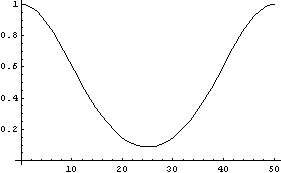
This is the condition that generated the SmoothData::bigsigma message above. Since the standard deviation of the Gaussian scales as the square root of the number of points in each data subset, the message can often be suppressed by reducing the number of points using the Points option.

6.2.3 How LoessFit Works

This section discusses the details of LoessFit, and in particular why it works so well as a data smoother and a nonparametric fitter. We will do a LoessFit to the ganglion data we have looked at before.

In[1]:=

In[2]:=

In[3]:=

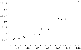
In[4]:=

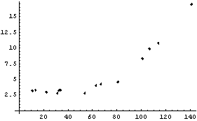
First, LoessFit divides the data into a number of partitions. For example, here is the eighth data point.

In[5]:=

Out[5]=

We shall examine the eight partition of the data set. In order to do this, we follow the progress of LoessFit in Subsubsection 6.2.3.1 below and define there the variables to be used here.Null

In[6]:=

In[7]:=

In[8]:=

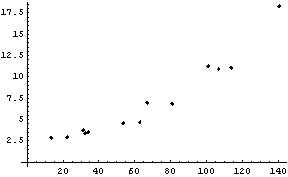
The weights for each value of the independent variable, as found in Subsubsection 6.2.3.1, are displayed.

In[9]:=

In[10]:=

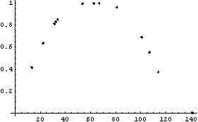
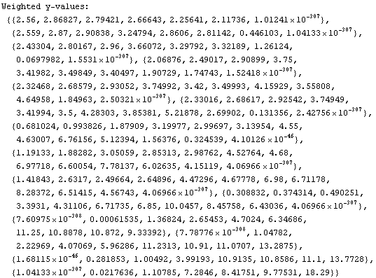
Next we look at the weighted data for this partition.

In[11]:=

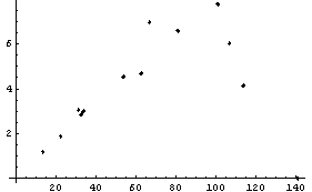
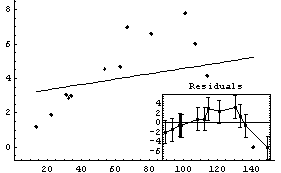
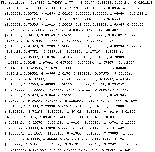
We fit this to a straight line.

In[12]:=

Out[12]=

Since we have chosen 13 points, the seventh member of this partition is the point we are trying to loess fit. Thus, the value that will replace the eighth value is calculated.

In[13]:=

Out[13]=

6.2.3.1 Digging Out Details From LoessFit

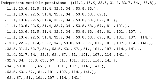
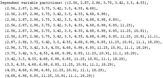
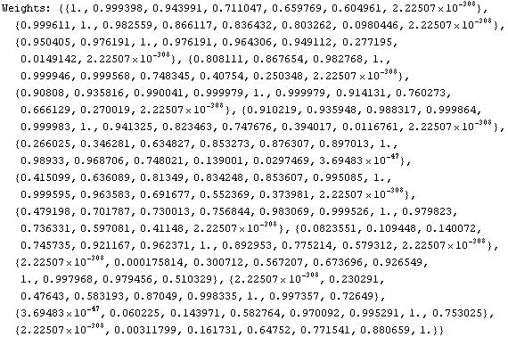
LoessFit accepts an option EDAShowProgress which provides many many details of its calculation. We will use that option to dig out the specifics we need in discussing how the program works.

In[1]:=