|
3.7.3 ACAnalysis

Command structure of ACAnalysis.
This functions allows for carrying out a numerical small-signal analysis. Given an AC DAEObject, ACAnalysis computes the small-signal solution in the specified frequency range and returns the result according to the Analog Insydes numerical data format described in Section 3.7.1. It consists of lists of rules, where the variables are assigned InterpolatingFunction objects.
The result of the small-signal analysis can be displayed with Analog Insydes graphics functions such as BodePlot.
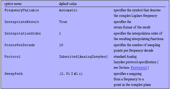
ACAnalysis has the following options:

Options for ACAnalysis.
See also: BodePlot, NoiseAnalysis, Section 3.7.1.
Options Description
A detailed description of all ACAnalysis options is given below in alphabetical order:
FrequencyVariable
This option specifies the symbol that denotes the complex Laplace frequency. See CircuitEquations in Section 3.5.1.
The default setting is FrequencyVariable -> Automatic, which means to use the symbol given in the DAEObject.
InterpolateResult
If InterpolateResult is set to True, the result is returned as an interpolating function for each variable. If the option is set to False, the result is returned as a list of {frequency, value} pairs.
InterpolationOrder
With InterpolationOrder -> integer you can change the interpolation order of the resulting interpolating functions (see the Mathematica object InterpolatingFunction).
The default setting is InterpolationOrder -> 1, which means linear interpolation.
PointsPerDecade
PointsPerDecade specifies the number of sampling points per frequency decade.
The default setting is PointsPerDecade -> 10.
SweepPath
SweepPath specifies a mapping from a frequency to a point in the complex plane. The option value has to be a pure function with one argument which returns a complex number.
The default setting is SweepPath -> (2. Pi I #1 &), which specifies a sweep along the  axis. axis.
Examples
Below we compute the frequency response of a RC lowpass filter circuit.
Load Analog Insydes.
In[1]:= <<AnalogInsydes`
Define netlist description.
In[2]:= lowpass =
Circuit[
Netlist[
{V1, {1, 0}, 1},
{R1, {1, 2}, 100.},
{C1, {2, 0}, 1.*^-6},
{R2, {2, 3}, 100.},
{C2, {3, 0}, 1.*^-6},
{RL, {3, 0}, 1000.}
]
]
Out[2]= 
Set up system of small-signal equations.
In[3]:= lowpasseqs = CircuitEquations[lowpass]
Out[3]= 
Display equations.
In[4]:= DisplayForm[lowpasseqs]
Out[4]//DisplayForm= 
Perform numerical small-signal analysis with ACAnalysis.
In[5]:= acsweep = ACAnalysis[lowpasseqs, {f, 1., 1.*^6}]
Out[5]= 
To solve only for one variable, specify the variable as second argument.
In[6]:= ACAnalysis[lowpasseqs, V$3, {f, 1., 1.*^6}]
Out[6]= 
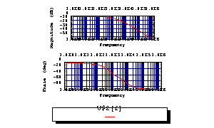
Display the simulation result with BodePlot.
In[7]:= BodePlot[acsweep, {V$2[f]}, {f, 1., 1.*^6}]

Out[7]= 
|