|
3.9.1 BodePlot

Command structure of BodePlot.
BodePlot displays one or several transfer functions in a Bode plot. A Bode plot consists of two separate charts in which the magnitude and phase of a transfer function are plotted vs. frequency. Magnitude and phase are displayed, respectively, on logarithmic and linear scales. The frequency axis is scaled logarithmically for both charts.
Note that BodePlot has attribute HoldFirst.
BodePlot supports additional patterns for displaying numerical data generated with the functions ACAnalysis, NoiseAnalysis, or ReadSimulationData:

Displaying numerical data with BodePlot.
You can customize the appearance of Bode plots with the options listed below. In addition, BodePlot inherits many options from LogLinearListPlot and Legend. Both the options which are specific to BodePlot as well as the inherited options can be set with SetOptions[BodePlot, opts].
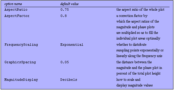
Options for BodePlot, Part I.
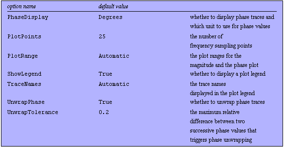
Options for BodePlot, Part II.
See also: ACAnalysis, NoiseAnalysis, ReadSimulationData, NicholPlot, NyquistPlot.
Options Description
A detailed description of all options that are specific to BodePlot or are used in a non-standard way is given below in alphabetical order:
FrequencyScaling
The option FrequencyScaling determines how sampling points are distributed over the frequency axis. Possible values are:

Values for the FrequencyScaling option.
MagnitudeDisplay
With the option MagnitudeDisplay, you can specify how magnitude values are displayed in a Bode plot. The following values are allowed:

Values for the MagnitudeDisplay option.
PhaseDisplay
The option PhaseDisplay specifies whether and how to display phase values. Possible choices are:

Values for the PhaseDisplay option.
PlotRange
With the PlotRange option, you can set the plot ranges for the  -axes of the magnitude and phase plots. Possible values are: -axes of the magnitude and phase plots. Possible values are:

Values for the PlotRange option.
TraceNames
The option TraceNames allows you to specify the labels that are shown in the plot legend for the displayed traces if ShowLegend -> True. The following values are possible:

Values for the TraceNames option.
UnwrapPhase
With the option UnwrapPhase, you can specify whether BodePlot should restrict phase values to the interval  or try to unwrap the phase values of a frequency response trace that wraps around the origin of the complex plane more than once. or try to unwrap the phase values of a frequency response trace that wraps around the origin of the complex plane more than once.
UnwrapTolerance
With UnwrapTolerance -> tol, you can specify the maximum percentage of a full  revolution by which two successive phase values may differ such that phase unwrapping is triggered. revolution by which two successive phase values may differ such that phase unwrapping is triggered.
Examples
Load Analog Insydes.
In[1]:= <<AnalogInsydes`
Define two transfer functions.
In[2]:= H1[s_] := 1/(s + 1);
H2[s_] := 10/(s^2 + s + 10)
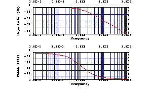
This produces a Bode plot of  . .
In[3]:= BodePlot[H1[I w], {w, 0.01, 100}]
Out[4]= 
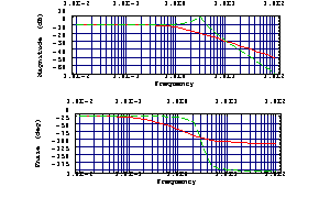
This produces a Bode plot of  and and  . .
In[4]:= BodePlot[{H1[I w], H2[I w]}, {w, 0.01, 100}]
Out[5]= 
This defines an RLC filter circuit.
In[5]:= rlcf = Netlist[
{V1, {1, 0}, Symbolic -> V, Value -> 1},
{R1, {1, 2}, Symbolic -> R1, Value -> 1000.},
{L1, {2, 3}, Symbolic -> L, Value -> 0.001},
{C1, {3, 0}, Symbolic -> C, Value -> 2.2*10^-6},
{R2, {3, 0}, Symbolic -> R2, Value -> 1000.}
];
Set up modified nodal equations.
In[6]:= eqsrlcf = CircuitEquations[rlcf]
Out[7]= 
Do an AC analysis from  to to  . .
In[7]:= acsweep = ACAnalysis[eqsrlcf, {f, 10, 10^6}]
Out[8]= 
Increase the number of plot points.
In[8]:= SetOptions[BodePlot, PlotPoints -> 200];
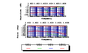
Display all traces in a Bode plot.
In[9]:= BodePlot[acsweep, {f, 10, 10^6}]
Out[10]= 
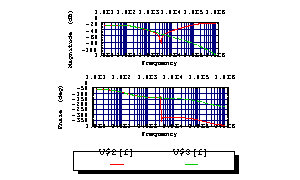
Display only the traces V$2[f] and V$3[f].
In[10]:= BodePlot[acsweep, {V$2[f], V$3[f]}, {f, 10, 10^6}]
Out[11]= 
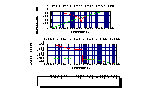
Display the traces V$2[f] and V$2[f]-V$3[f].
In[11]:= BodePlot[acsweep, {V$2[f], V$2[f]-V$3[f]}, {f, 10, 10^6}]
Out[12]= 
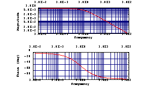
Show absolute magnitude values instead of decibels.
In[12]:= BodePlot[H1[I w], {w, 0.01, 100},
MagnitudeDisplay -> AbsoluteValues]
Out[13]= 
Show magnitude values on a linear scale.
In[13]:= BodePlot[H1[I w], {w, 0.01, 100},
MagnitudeDisplay -> Linear]
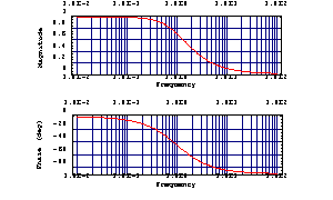
Out[14]= 
Do not show the phase plot.
In[14]:= BodePlot[acsweep, {V$2[f], V$2[f]-V$3[f]},
{f, 100, 10^5}, PhaseDisplay -> None]
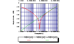
Out[15]= 
Restrict the phase to the interval  . .
In[15]:= BodePlot[H1[I w]^5, {w, 0.01, 100}, UnwrapPhase -> False]
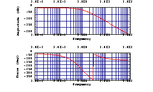
Out[16]= 
Unwrap the phase trace.
In[16]:= BodePlot[H1[I w]^5, {w, 0.01, 100}, UnwrapPhase -> True]
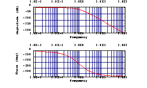
Out[17]= 
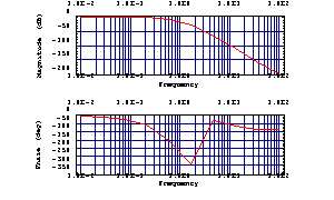
In the following example, the number of plot points is reduced so that the differences between successive phase values become too large for phase unwrapping.
Reduce the number of plot points.
In[17]:= BodePlot[H1[I w]^5, {w, 0.01, 100},
PlotPoints -> 10, PlotRange -> {Automatic, {-360, 0}}]
Out[18]= 
To unwrap the phase trace, you can specify a larger number of plot points or increase the value of UnwrapTolerance.
Increase the unwrap tolerance to 30% of  . .
In[18]:= BodePlot[H1[I w]^5, {w, 0.01, 100},
PlotPoints -> 10, UnwrapTolerance -> 0.3]

Out[19]= 
|