|
3.9.3 NicholPlot

Command structure of NicholPlot.
NicholPlot displays one or several transfer functions in a Nichol plot. A Nichol plot is similar to a Nyquist plot but shows magnitude (in dB) vs. phase with the axis origin at the point  . .
Note that NicholPlot has attribute HoldFirst.
NicholPlot supports additional patterns for displaying numerical data generated with the functions ACAnalysis, NoiseAnalysis, or ReadSimulationData:

Displaying numerical data with NicholPlot.
You can customize the appearance of Nichol plots with the following options. In addition, NicholPlot inherits many options from ListPlot and Legend. Both the options which are specific to NicholPlot as well as the inherited options can be set with SetOptions[NicholPlot, opts].

Options for NicholPlot.
See also: ACAnalysis, NoiseAnalysis, ReadSimulationData, BodePlot, NyquistPlot.
Options Description
A detailed description of all options that are specific to NicholPlot or are used in a non-standard way is given below in alphabetical order:
FrequencyScaling
The option FrequencyScaling determines how sampling points are distributed over the frequency axis. Possible values are:

Values for the FrequencyScaling option.
PhaseDisplay
The option PhaseDisplay specifies the unit for phase values. Possible values are:

Values for the PhaseDisplay option.
TraceNames
The option TraceNames allows you to specify the labels that are shown in the plot legend for the displayed traces if ShowLegend -> True. The following values are possible:

Values for the TraceNames option.
Examples
Load Analog Insydes.
In[1]:= <<AnalogInsydes`
Define two transfer functions.
In[2]:= H1[s_] := (60 + 20*s)/(100*s + 45*s^2 + 15*s^3 + 2*s^4)
H2[s_] := 10/(s^2 + s + 10)
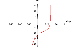
Draw a Nichol plot of  . .
In[3]:= NicholPlot[H1[I w], {w, 0.1, 5}, AspectRatio -> 0.8]

Out[4]= 
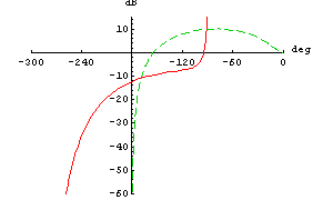
Display two transfer functions in a Nichol plot.
In[4]:= NicholPlot[{H1[I w], H2[I w]}, {w, 0.1, 100},
AspectRatio -> 0.7, PlotRange -> {{-300,0}, {-60,15}},
PlotPoints -> 100]

Out[5]= 
This defines an RLC filter circuit.
In[5]:= rlcf = Netlist[
{V1, {1, 0}, Symbolic -> V, Value -> 1},
{R1, {1, 2}, Symbolic -> R1, Value -> 1000.},
{L1, {2, 3}, Symbolic -> L, Value -> 0.001},
{C1, {3, 0}, Symbolic -> C, Value -> 2.2*10^-6},
{R2, {3, 0}, Symbolic -> R2, Value -> 1000.}
];
Set up modified nodal equations.
In[6]:= eqsrlcf = CircuitEquations[rlcf]
Out[7]= 
Do an AC analysis from  to to  . .
In[7]:= acsweep = ACAnalysis[eqsrlcf, {f, 10, 10^6}]
Out[8]= 
Display several expressions in a Nichol plot.
In[8]:= NicholPlot[acsweep, {V$2[f], V$3[f]}, {f, 10, 10^6},
AspectRatio -> 0.8]

Out[9]= 
|