3.9.4 NyquistPlot

Command structure of NyquistPlot.

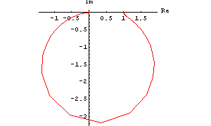
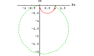
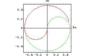
NyquistPlot displays one or several transfer functions in a Nyquist plot. A Nyquist plot is a parametric plot of the imaginary part vs. the real part of a frequency response as the frequency is swept from to .

Note that NyquistPlot has attribute HoldFirst.

NyquistPlot supports additional patterns for displaying numerical data generated with the functions ACAnalysis, NoiseAnalysis, or ReadSimulationData:

Displaying numerical data with NyquistPlot.

You can customize the appearance of Nyquist plots with the following options. In addition, NyquistPlot inherits many options from ListPlot and Legend. Both the options which are specific to NyquistPlot as well as the inherited options can be set with SetOptions[NyquistPlot, opts].

Options for NyquistPlot.

See also: ACAnalysis, NoiseAnalysis, ReadSimulationData, BodePlot, NicholPlot.

Options Description

A detailed description of all options that are specific to NyquistPlot or are used in a non-standard way is given below in alphabetical order:

FrequencyScaling

The option FrequencyScaling determines how sampling points are distributed over the frequency axis. Possible values are:

Values for the FrequencyScaling option.

ShowUnitCircle

With ShowUnitCircle -> True, NyquistPlot adds the unit circle to a plot.

TraceNames

The option TraceNames allows you to specify the labels that are shown in the plot legend for the displayed traces if ShowLegend -> True. The following values are possible:

Values for the TraceNames option.

UnitCircleStyle

With UnitCircleStyle -> style, you can change the plot style for the unit circle.

Examples

Load Analog Insydes.

In[1]:= <<AnalogInsydes`

Define two transfer functions.

In[2]:= H1[s_] := 1/(s + 1);
H2[s_] := 10/(s^2 + s + 10)

Increase the number of plot points.

In[3]:= SetOptions[NyquistPlot, PlotPoints -> 200];

Draw a Nyquist plot of .

In[4]:= NyquistPlot[H2[I w], {w, 0.01, 100}, PlotRange -> All]

Out[5]=

This produces a Nyquist plot of and .

In[5]:= NyquistPlot[{H1[I w], H2[I w]}, {w, 0.01, 100},
PlotRange -> All]

Out[6]=

This defines an RLC filter circuit.

In[6]:= rlcf = Netlist[
{V1, {1, 0}, Symbolic -> V, Value -> 1},
{R1, {1, 2}, Symbolic -> R1, Value -> 1000.},
{L1, {2, 3}, Symbolic -> L, Value -> 0.001},
{C1, {3, 0}, Symbolic -> C, Value -> 2.2*10^-6},
{R2, {3, 0}, Symbolic -> R2, Value -> 1000.}
];

Set up modified nodal equations.

In[7]:= eqsrlcf = CircuitEquations[rlcf]

Out[8]=

Do an AC analysis from to .

In[8]:= acsweep = ACAnalysis[eqsrlcf, {f, 10, 10^6}]

Out[9]=

Display the trace of V$2[f].

In[9]:= NyquistPlot[acsweep, {V$2[f]}, {f, 10, 10^6}]

Out[10]=

Display several expressions in a Nyquist plot.

In[10]:= NyquistPlot[acsweep, {V$2[f]-0.5, 0.5-V$2[f]},
{f, 10, 10^6}, Frame -> True, ShowLegend -> False]

Out[11]=

Display the unit circle.

In[11]:= NyquistPlot[H2[I w], {w, 0.01, 100},
PlotRange -> {{-3, 3}, {-3.5, 1.5}},
ShowUnitCircle -> True]

Out[12]=

Display the unit circle using a different style.

In[12]:= NyquistPlot[H2[I w], {w, 0.01, 100},
PlotRange -> {{-3, 3}, {-3.5, 1.5}},
ShowUnitCircle -> True,
UnitCircleStyle ->
{GrayLevel[0], Dashing[{0.04, 0.03}]}]

Out[13]=