|
3.7.5 NDAESolve

Command structure of NDAESolve.
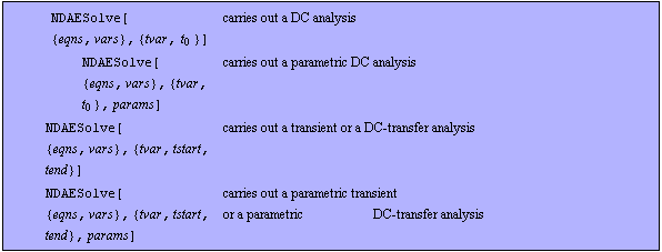
The function NDAESolve allows for carrying out several numerical analyses, such as an operating-point (DC) analysis, a DC-transfer (DT) analysis, or a large-signal (transient) analysis. NDAESolve returns the result according to the Analog Insydes numerical data format described in Section 3.7.1. It consists of lists of rules, where the variables are assigned InterpolatingFunction objects in case of a transient analysis or numerical values in case of a DC analysis. Both analysis modes can also be carried out as parametric analyses. For this, specify a parameter sweep params according to the Analog Insydes parameter sweep format described in Section 3.7.2.
The result of the numerical transient analysis can be displayed with Analog Insydes graphics functions such as TransientPlot.
Note that NDAESolve still supports the command structure from Release 1 where the first argument is given as {eqns, vars} instead of a DAEObject:
Additional patterns of NDAESolve.
NDAESolve has the following options:

Nonlinear solver options of NDAESolve.

Step size control options of NDAESolve.

Operating-point computation options of NDAESolve.

Return format options of NDAESolve.

Miscellaneous options of NDAESolve.
See also: TransientPlot, Section 3.7.1, Section 3.7.2.
Options Description
A detailed description of all NDAESolve options is given below in alphabetical order:
AnalysisMode
The option AnalysisMode specifies the circuit analysis mode, where the default setting is AnalysisMode -> Transient. Valid option values are as follows:

Values for the AnalysisMode option.
Note that this option is only valid for the NDAESolve pattern where you have to specify a start value tstart and an end value tend. In this case NDAESolve is able to carry out a DC-transfer analysis by setting the option to AnalysisMode -> DC, although the input is a Transient DAEObject.
Note that the DC-transfer analysis method replaces all derivatives in the circuit equations by zero. Thus, inductors are replaced by short circuits because all inductor voltages are set to zero:

and capacitors are replaced by open circuits because all capacitor currents are set to zero:

BreakOnError
The option BreakOnError allows for interrupting a parametric DC or transient analysis in case of an error. If set to True and the computation for one parameter sweep fails, the simulation is interrupted and $Failed is returned. The default setting is BreakOnError -> False.
CompressEquations
The option CompressEquations allows for carrying out a symbolic pre-processing of the equation system before it is solved numerically. This means that equations and variables which are not relevant for computing the variables of interest (given by the option OutputVariables) are removed. Note that this option is only effective if the option OutputVariables is not set to All. The option is realized by an internal call of the function CompressNonlinearEquations. The default setting is CompressEquations -> False.
DesignPoint
With DesignPoint -> { -> ->  , ,  } you can overwrite the design point given in the DAEObject (see also CircuitEquations in Section 3.5.1). The default setting is DesignPoint -> Automatic, which means to use the design point given in the DAEObject. } you can overwrite the design point given in the DAEObject (see also CircuitEquations in Section 3.5.1). The default setting is DesignPoint -> Automatic, which means to use the design point given in the DAEObject.
InitialConditions
The option InitialConditions allows for considering initial conditions (see also CircuitEquations in Section 3.5.1). The default setting is InitialConditions -> Automatic. Valid option values are as follows:

Values for the InitialConditions option.
InitialGuess
The option InitialGuess allows for explicitly specifying an initial guess for the Newton iteration when computing the operating point. Note that missing variables are set to zero. The default setting is InitialGuess -> Automatic, which means that all variables have the initial value zero. Possible option values are as follows:

Values for the InitialGuess option.
InitialSolution
The option InitialSolution allows for specifying an initial solution for certain variables of the operating point. Note that missing variables are computed consistently. The default setting is InitialSolution -> Automatic, which automatically computes the operating point. Possible option values are as follows:

Values for the InitialSolution option.
InterpolationOrder
With InterpolationOrder -> integer you can change the interpolation order of the resulting interpolating functions (see the Mathematica object InterpolatingFunction). The default setting is InterpolationOrder -> 1, which means linear interpolation.
MaxDelta
One of the conditions included in the automatic step size control is a check for rapidly changing variable values from a certain point in time to its succeeding time instant. The maximum allowed deviation is controlled via the option MaxDelta. The default setting is MaxDelta -> 1.
MaxIterations
MaxIterations specifies the maximum number of iterations the nonlinear equation solver should use attempting to find a solution. The option setting can either be an integer int or a list of two integers { , ,  }. If it is specified as a single integer int then it is equivalent to the list {int, int}. The first integer value defines the iteration limit for finding a DC operating-point and the second integer value the iteration limit for transient computations, respectively. If the number of iterations for the operating-point computation exceeds the limit, an error message is generated and the computation is interrupted. If the iteration limit for transient computations is exceeded, the step size is reduced by the factor given by the option StepSizeFactor. The default setting is MaxIterations -> {100, 20}. }. If it is specified as a single integer int then it is equivalent to the list {int, int}. The first integer value defines the iteration limit for finding a DC operating-point and the second integer value the iteration limit for transient computations, respectively. If the number of iterations for the operating-point computation exceeds the limit, an error message is generated and the computation is interrupted. If the iteration limit for transient computations is exceeded, the step size is reduced by the factor given by the option StepSizeFactor. The default setting is MaxIterations -> {100, 20}.
MaxSteps
The option MaxSteps limits the number of integration steps. The computation will be stopped immediately if the limiting value is exceeded. The default setting is MaxSteps -> Automatic, which means  . .
MaxStepSize
The option MaxStepSize specifies the upper limit of the integration step size. The default setting is MaxStepSize -> Automatic, which means  . .
MinStepSize
The option MinStepSize specifies the lower limit of the integration step size. The computation will be stopped immediately if the integration step size falls below this limit. The default setting is MinStepSize -> Automatic, which means  . .
NonlinearMethod
The option NonlinearMethod allows for choosing between different algorithms for numerically solving nonlinear equation systems. The default setting is NonlinearMethod -> FindRoot. Valid option values are as follows:

Values for the NonlinearMethod option.
OutputVariables
The option OutputVariables specifies those variables which should be included in the solution vector. The default setting is OutputVariables -> All. Valid option values are as follows:

Values for the OutputVariables option.
RandomFunction
The option RandomFunction specifies a function used for generating random numbers for perturbing the initial guess during the operating-point computation. Note that the generated random numbers are added to the initial guess. The return value of the function should be a real number. The default setting is RandomFunction -> (Random[Real, {0., 0.1}]&).
ReturnDerivatives
The option ReturnDerivatives allows for including solutions of the derivatives in the solution vector. The default setting is ReturnDerivatives -> False.
Simulator
The option Simulator specifies the simulator which should be applied for numerically solving the system of equations. The default setting is Simulator -> Inherited[AnalogInsydes]. Valid option values are as follows:

Values for the Simulator option.
In case of an external simulator kernel a behavioral model in the simulator-specific language is generated with the function WriteModel. Then the respective simulator kernel given by the option SimulatorExecutable is applied, and finally the generated simulation data is imported via the function ReadSimulationData.
Please note that this option is in an experimental state. Additionally, it is extremely dependent on the applied simulator, its underlying operating system, and even the available simulator version.
SimulatorExecutable
The option SimulatorExecutable specifies the name of the external simulator executable. Note that this option is only effective if an external simulator is applied via the option Simulator. The default setting is SimulatorExecutable -> Automatic, which means "pspice" in case of PSpice and "saber" in case of Saber, respectively. If set to a string make sure that the simulator call corresponds to the setting of the Simulator option. Otherwise the internal calls to the functions WriteModel and ReadSimulationData fail. Valid option values are as follows:

Values for the SimulatorExecutable option.
StartingStepSize
The option StartingStepSize specifies the initial integration step size. The default setting is StartingStepSize -> Automatic, which means  . .
StepSizeFactor
To speed up the computation time NDAESolve includes an automatic step size control. If the deviations of the variable values from one time point to its succeeding time instant fulfill certain conditions the actual step size will be multiplied or divided by the value given by the option StepSizeFactor. The default setting is StepSizeFactor -> 1.5.
Examples
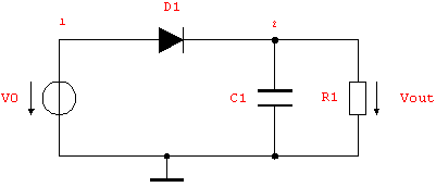
Consider the following diode rectifier circuit with a sinusoidal input voltage.
Load Analog Insydes.
In[1]:= <<AnalogInsydes`
Define netlist description of a simple diode rectifier circuit.
In[2]:= rectifier =
Circuit[
Netlist[
{V0, {1, 0}, Symbolic -> V0,
Value -> 2. Sin[10^6 Time]},
{R1, {2, 0}, Symbolic -> R1, Value -> 100.},
{C1, {2, 0}, Symbolic -> C1, Value -> 1.*^-7},
{D1, {1 -> A, 2 -> C},
Model -> "Diode", Selector -> "Spice"}
]
]
Out[2]= 
Set up system of symbolic time-domain equations.
In[3]:= rectifiereqs = CircuitEquations[rectifier,
AnalysisMode -> Transient, ElementValues -> Symbolic]
Out[3]= 
Display equations.
In[4]:= DisplayForm[rectifiereqs]
Out[4]//DisplayForm= 
Perform numerical DC analysis with NDAESolve.
In[5]:= NDAESolve[rectifiereqs, {t, 0.}]
Out[5]= 
Perform numerical transient analysis with NDAESolve.
In[6]:= tran = NDAESolve[rectifiereqs, {t, 0., 2.*^-5}]
Out[6]= 
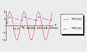
Display the simulation result.
In[7]:= TransientPlot[tran, {V$1[t], V$2[t]}, {t, 0., 2.*^-5}]
Out[7]= 
Perform numerical DC-transfer analysis with NDAESolve.
In[8]:= dctran = NDAESolve[rectifiereqs, {t, 0., 1.*^-5},
AnalysisMode -> DC]
Out[8]= 
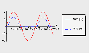
Display the simulation result.
In[9]:= TransientPlot[dctran, {V$1[t], V$2[t]}, {t, 0., 1.*^-5}]
Out[9]= 
Perform parametric transient analysis with NDAESolve.
In[10]:= paramtran = NDAESolve[rectifiereqs, {t, 0., 2.*^-5},
{R1, Table[10^i, {i, 0, 3}]}]
Out[10]= 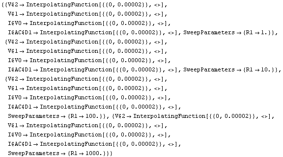
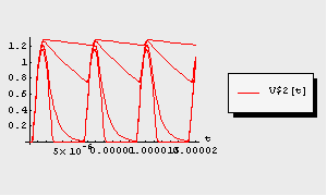
By default, TransientPlot displays the solutions for all parameter sweep values within a single plot.
Display the simulation result.
In[11]:= TransientPlot[paramtran, {V$2[t]}, {t, 0., 2.*^-5}]
Out[11]= 
Consider the following oscillator circuit with initial conditions at the time  . .
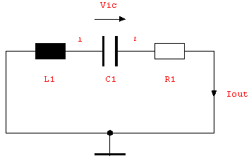
Define netlist description of a simple oscillator circuit.
In[12]:= oscillator =
Netlist[
{L1, {0, 1}, Symbolic -> L1, Value -> 1.*^-5},
{C1, {1, 2}, Symbolic -> C1, Value -> 3.*^-7,
InitialCondition -> 2.*^-3},
{R1, {2, 0}, Symbolic -> R1, Value -> 1.}
]
Out[12]= 
Set up system of symbolic time-domain equations with initial conditions where given in the netlist.
In[13]:= oscillatoreqs1 = CircuitEquations[oscillator,
AnalysisMode -> Transient, ElementValues -> Symbolic,
InitialConditions -> Automatic];
DisplayForm[oscillatoreqs1]
Out[14]//DisplayForm= 
Set up system of symbolic time-domain equations with initial conditions for all dynamic netlist elements.
In[14]:= oscillatoreqs2 = CircuitEquations[oscillator,
AnalysisMode -> Transient, ElementValues -> Symbolic,
InitialConditions -> All];
DisplayForm[oscillatoreqs2]
Out[16]//DisplayForm= 
Perform numerical transient analysis for both equation systems.
In[15]:= tran1 = NDAESolve[oscillatoreqs1, {t, 0., 1.*^-4}];
tran2 = NDAESolve[oscillatoreqs2, {t, 0., 1.*^-4}];
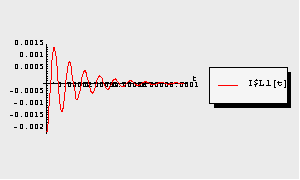
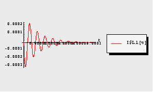
With InitialConditions -> Automatic, initial conditions are applied only where specified in the netlist, all others are computed consistently. With InitialConditions -> All, initial conditions are set to zero for all elements for which there is no condition specified in the netlist. You can see the difference between both possibilities in the following two plots.
Display the first simulation result.
In[16]:= TransientPlot[tran1, {I$L1[t]}, {t, 0., 1.*^-4},
PlotRange -> All]
Out[19]= 
Display the second simulation result.
In[17]:= TransientPlot[tran2, {I$L1[t]}, {t, 0., 1.*^-4}]
Out[20]= 
|