7.2 Static Solutions

Load objects are applied to the current model with the SetLoads function. The actual load vector developed by SetLoads is not returned to the user, rather it is stored in several variables in the `Private` context of the Mech packages. The use of load objects and SetLoads in Mech is analogous to the use of constraint objects and SetConstraints.
Mech uses a Lagrange multiplier method to resolve the constraint reaction forces in a mechanism model. There is one Lagrange multiplier named 1, 2, and so on for each degree of freedom in the model. Thus, when Mech solves a loaded model what is returned to the user are the numerical values of the Lagrange multipliers. The Lagrange multipliers are actually the generalized forces related to a set of generalized coordinates in which each coordinate corresponds to the magnitude of the violation of a kinematic constraint.
While the numerical values of the Lagrange multipliers are not directly very useful, they are converted into the reaction forces and moments that are applied by the constraints to each body in the model with the Reaction function. This is discussed in Section 7.3.

7.2.1 2D Example Mechanism

To demonstrate the use of Mech's static force solution method a 2D model is developed that is subject to applied loads. A 3D model would be treated in the same manner as 2D with regard to the application of forces. The model is a simple ladder sliding down a wall consisting of one moving body, the ladder.
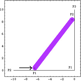
The input to the mechanism is to push the bottom of the ladder across the horizontal floor, in either direction. The ladder is constrained such that the bottom of the ladder must contact the floor and the top of the ladder must contact the vertical wall.

This loads the Modeler2D package.

In[1]:=

Here is a graphic of the 2D ladder-on-wall model.

Bodies

Two body objects are defined for the ladder-on-wall model.

Names are defined for each of the body numbers in the model.

In[2]:=

Here are the body objects for the ladder-on-wall model.

In[4]:=

SetBodies incorporates the body properties into the current model.

In[6]:=

Constraints

Three constraints, one of which is a driving constraint, are required to model the ladder-on-wall. The top and bottom tips of the ladder, which slide on the wall and floor, each have a small radius.

Here are the constraint objects for the ladder-on-wall model.

In[7]:=

SetConstraints incorporates the constraint objects into the current model.

In[10]:=

7.2.2 Applying Loads

SetLoads is the core function for applying loads to a Mech model. SetLoads takes load objects that represent the physical loads applied to the model and builds them into a global load vector that represents the total force and moment applied at the origin of each body in the model.

The load application function.

Mech uses a Lagrange multiplier method to resolve the static and dynamic forces on a model, which will be discussed further in Section 7.3. It is usually not necessary to specify initial guesses for the Lagrange multipliers, because the equations of motion are linear in the Lagrange multipliers unless friction forces are applied. If initial guesses are needed, they can be specified with the LambdaGuess option for SetLoads.

An option for SetLoads.

Because forces and moments are additive quantities, it is not necessary to apply all of the loads to the model simultaneously. With the AddLoads option, loads can be applied to the model sequentially.

An option for SetLoads.

Loads for the Model

Three loads are defined for the model developed in Section 7.2.1.

Here are the load objects for the ladder-on-wall model.

In[11]:=

Out[13]=

Initially, only the two Force objects are applied. SetLoads incorporates the loads into the model.

In[14]:=

By using the AddLoads option for SetLoads, additional loads can be applied to the model at any time. Thus, the Moment can simply be added to the current loading.

This adds the Moment object to the ladder-on-wall model.

In[15]:=

Mech load objects can contain dependencies on other dependent variables. For example, to model the force applied by a linear spring, it is necessary to have the magnitude of the force be a function of the distance between two points.
The Force of an extension spring with a free length of 2 units and a spring constraint k attached between the top of the ladder and the top of the wall could be modeled as follows.

Here is a spring force.

In[16]:=

7.2.3 Running the Loaded Model

Because of the presence of T in the driving constraint cs[1], the model can be run through its intended range of motion by varying T directly with the SolveMech command. The numerical value of T specifies the distance between the bottom of the ladder and the wall.
Although loads have been added to the model, the SolveMech default option setting Solution -> Location solves only for the location variables.

Now run the model at T = 7.5.

In[17]:=

Out[17]=

Mech must be told to solve for the static forces in the model with the Solution option for SolveMech.

An option for SolveMech.

The Solution -> Static option causes SolveMech to resolve the forces applied to the model into Lagrange multipliers.

Now run the model at T = 8.5.

In[18]:=

Out[18]=

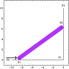
Here is the ladder-on-wall image at T = 8.5.

The numeric values of the Lagrange multipliers returned by SolveMech are not directly very useful, unless one has a very good understanding of the exact form of the constraints. However, the set of Lagrange multipliers associated with a mechanism model completely determines all of the reaction forces in the constraints in the model. To find the actual reaction forces and moments at a specific constraint it is necessary to use the Mech Reaction function, which is described in Section 7.3.

Undocumented Graphics Generation