3.1 2D Output FunctionsNumerical output from a Modeler2D model can be generated with output functions that are defined in the auxiliary package Graphics2D. This package is autoloaded after the Modeler2D main package has been loaded if any of the output functions are called. Each output function returns a symbolic expression that represents the quantity being sought, in terms of the model's dependent variables, X2, Y3, and so on. To achieve a numerical result, the dependent variables must be replaced with numbers, usually by applying a solution rule returned by SolveMech. More complicated and specific output functions can easily be defined by the user, making use of Mech's basic output functions and Mathematica's built-in vector algebra functions. 3.1.1 Example Mechanism To demonstrate the use of Modeler2D output functions, a 2D model is developed that can have various geometric quantities measured. The model is a planar quick-return mechanism consisting of three moving bodies: the crank, drive arm, and slider. A real quick-return mechanism would have a fourth body, the connecting rod between the drive arm and the slider, but this body is simply modeled with a relative-distance constraint.
The motion of the quick-return mechanism is driven by the rotation of the crank that, in turn, forces the drive arm to rock about its lower pivot point on the ground, via a pin on the crank that slides in a straight slot on the drive arm. The top of the drive arm is attached to a connecting rod, which is attached to the slider, which slides on horizontal path on the ground. This loads the Modeler2D package. Here is a graphic of the 2D quick-return model.
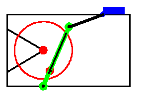
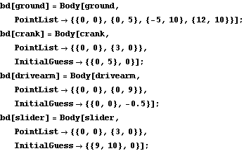
BodiesFour body objects are defined for the quick-return mechanism model. The ground (body 1) requires four point definitions.
P1 is the rotational axis of the drive arm.
P2 is the rotational axis of the crank.
P3 and P4 are two points that define the line upon which the slider slides.The crank (body 2) requires two local point definitions.
P1 is the crank's rotational axis.
P2 is the location of the pin on the crank that engages with the drive arm.The drive arm (body 3) requires two local point definitions.
P1 is the point on the drive arm where the drive arm pivots with respect to the ground.
P2 is the point where the drive arm is attached to the pseudo-connecting rod.The slider (body 4) requires two local point definitions.
P1 and P2 are two points along the horizontal axis of the slider define its translation line.Here are the bodies in the quick-return model.
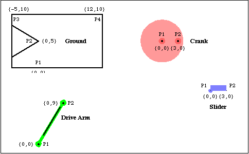
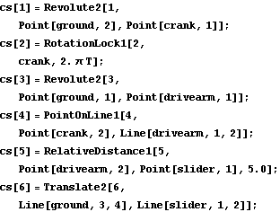
Names are defined for each of the body numbers in the mechanism. Body objects are defined for each body. This incorporates the body properties into the current model. ConstraintsFive constraints and one driving constraint are required to model the quick-return mechanism. A Revolute2 constraint forces the axis of the crank to be coincident with its pivot point on the ground. This constrains two degrees of freedom, X and Y displacement of the crank axis.A RotationLock1 constraint specifies the angular coordinate of the crank. This driving constraint is used to rotate the crank.A Revolute2 constraint forces the lower pivot point of the drive arm to be coincident with the global origin. The drive arm can pivot about this point on the ground.A PointOnLine1 constraint between the crank and the drive arm where the pin on the crank slides in a slot on the drive arm.A RelativeDistance1 constraint between the drive arm and the slider replaces the pseudo-connecting rod, which is 5.0 units long.A Translate2 constraint between the slider and the ground allows the slider to translate horizontally along a track on the ground.Here are five constraints for the quick-return model. This incorporates the constraints into the current model. RuntimeThis runs the model at T = 0.15
Out[18]= |  |
Here is the quick-return mechanism at T = 0.15.
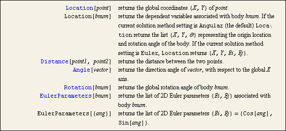
3.1.2 Output FunctionsModeler2D numerical output functions return expressions that evaluate to numbers or vectors, such as the distance between two points, the angle between two lines, or the coordinates of a point. These functions take point, vector, and axis objects as arguments, identical in structure to the geometry objects used when building constraints. When local point numbers are used, the local coordinates are taken from the current body objects, as specified with SetBodies.
Each of the output functions are demonstrated in the context of the quick-return mechanism model defined in Section 3.1.1. Output functions. More complex output functions. The Location function is used to convert a Mech Point object into the global coordinates of the point. Here are the global coordinates of point 2 on the drive arm.
Out[19]= |  |
Location assumes a point object if only the arguments of Point are given.
Out[20]= |  |
This gets a numerical result from the output of Location.
Out[21]= |  |
Out[22]= |  |
The Distance function is used to find the absolute distance between any two points in space. The points can be on one body or on two different bodies. Here is the distance from the center of the crank to point 2 on the slider.
Out[23]= |  |
Here is the numerical result.
Out[24]= |  |
Here is the length of the line from the center of the crank to the drive pin.
Out[25]= |  |
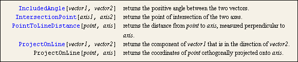
Note that it was not necessary to apply a solution rule to the last example to get a numerical result because the dimension being measured is not a function of the coordinates of each body. Here is the minimum distance between the crank axis and the center line of the drive arm.
Out[26]= |  |
Now get a numerical result.
Out[27]= |  |
Note that the distance is zero when the crank has turned 1/4 turn, and the drive arm is pointed straight up, through the axis of the crank. Here is the direction angle of the center line of the connecting rod.
Out[28]= |  |
Now get a numerical result in degrees.
Out[29]= |  |
The Rotation function simply returns the angular coordinate of the specified body. Here is theta of the drive arm.
Out[30]= |  |
This returns the intersection of the connecting rod axis and a vertical line through the crank axis.
Out[31]= |  |
The ProjectOnLine function is used to find the projection of a point on one body onto a line located on another body (or bodies). This projects the crank's drive pin onto the connecting rod.
Out[32]= |  |
3.1.3 Vector Algebra FunctionsModeler2D vector algebra functions perform many common vector algebra operations such as cross and dot products of vectors. These functions can be used to build more complicated functions that are not provided by Modeler2D. The output functions take point, vector, and axis objects as arguments, identical in structure to the geometry objects used when building constraint objects. When local point numbers are used, the local coordinates are taken from the current body objects, as specified with SetBodies.
Each of the vector algebra functions are demonstrated in the context of the quick-return mechanism model defined at the beginning of this section. Vector algebra functions. The Direction function is used to convert Modeler2D vector objects into 2D vectors in global coordinates. Note that Mech's definition of Direction does not interfere with its use as a built-in Mathematica symbol. Here is the direction vector of the connecting rod.
Out[33]= |  |
Now get a numerical result.
Out[34]= |  |
Several Modeler2D output functions are textbook vector algebra functions that are capable of dealing with normal 2D vectors or Modeler2D line objects interchangeably. Magnitude can return the length of the line from one end of the connecting rod to the other.
Out[35]= |  |
Magnitude also works with simple vectors.
Out[36]= |  |
Unit also works with vectors or line objects.
Out[37]= |  |
The cross product of two vectors in 2D space is a scalar.
Out[38]= |  |
Now get a numerical result.
Out[39]= |  |
Here is a 2D rotation matrix that will rotate a vector on the slider into global coordinates.
Out[40]= |  |
The global coordinates of a point specified in a local reference frame are equal to the coordinates of the origin of the reference frame plus the local coordinates of the point, rotated into the global reference frame. Here is a calculation of the global coordinates of the local point {3, 8} on the slider.
Out[41]= |  |
The Location function performs effectively the same calculation, directly.
Out[42]= |  |
Now get a numerical result.
Out[43]= |  |
The PointToLocal function converts the global point back to local coordinates.
Out[44]= |  |
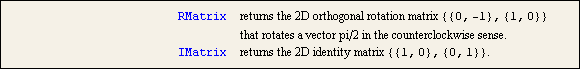
Two constant matrices that are commonly used in 2D vector algebra are also defined by Modeler2D. Constant utilities. Coordinate ConversionsPolarToXY and XYToPolar are two conversion functions that do not accept Modeler2D geometry objects as arguments. These functions only accept 2D vectors of the form {x, y}. Coordinate conversions. This converts a polar coordinate pair to Cartesian coordinates.
Out[45]= |  |
This converts it back.
Out[46]= |  |
This converts a 2D vector to polar coordinates.
Out[47]= |  |
|